46—Chapter 19. Additional Regression Tools

are said to be non-identified if there are multiple sets of coefficients which identically yield the minimized sum-of-squares value. If this condition holds, it is impossible to choose between the coefficients on the basis of the minimum sum-of-squares criterion.

is not identified, since any coefficient pair (b1, b2) is indistinguishable from the pair (–b1, –b2 ) in terms of the sum-of-squared residuals.

For a thorough discussion of identification of nonlinear least squares models, see Davidson and MacKinnon (1993, Sections 2.3, 5.2 and 6.3).

Convergence Criterion

EViews may report that it is unable to improve the sums-of-squares. This result may be evidence of non-identification or model misspecification. Alternatively, it may be the result of setting your convergence criterion too low, which can occur if your nonlinear specification is particularly complex.

If you wish to change the convergence criterion, enter the new value in the Options tab. Be aware that increasing this value increases the possibility that you will stop at a local minimum, and may hide misspecification or non-identification of your model.

See “Setting Estimation Options” on page 751, for related discussion.

Stepwise Least Squares Regression

EViews allows you to perform automatic variable selection using stepwise regression. Stepwise regression allows some or all of the variables in a standard linear multivariate regression to be chosen automatically, using various statistical criteria, from a set of variables.

There is a fairly large literature describing the benefits and the pitfalls of stepwise regression. Without making any recommendations ourselves, we refer the user to Derksen and Keselman (1992), Roecker (1991), Hurvich and Tsai (1990).

Stepwise Least Squares Estimation in EViews

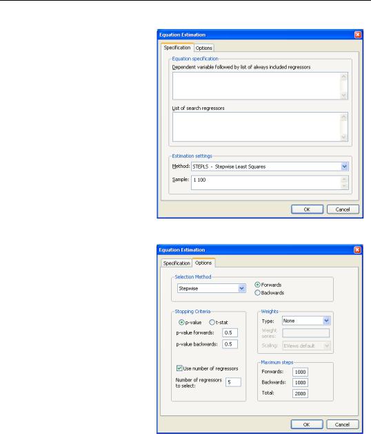
To perform a Stepwise selection procedure (STEPLS) in EViews select Object/New Object/ Equation, or press Estimate from the toolbar of an existing equation. From the Equation Specification dialog choose Method: STEPLS - Stepwise Least Squares. EViews will display the following dialog:

48—Chapter 19. Additional Regression Tools

ber of regressors by selecting the Use number of regressors option and providing a number of the corresponding edit field.

You may also set the maximum number of steps taken by the procedure. To set the maximum number of additions to the model, change the Forwards steps, and to set the maximum number of removals, change the Backwards steps. You may also set the total number of additions and removals. In general it is best to leave these numbers at a high value. Note, however, that the Stepwise routines have the potential to repetitively add and remove the same variables, and by setting the maximum number of steps you can mitigate this behavior.

The Swapwise method lets you choose whether you wish to use Max R-squared or Min R- squared, and choose the number of additional variables to be selected. The Combinatorial method simply prompts you to provide the number of additional variables. By default both of these procedures have the number of additional variables set to one. In both cases this merely chooses the single variable that will lead to the largest increase in R-squared.

For additional discussion, see “Selection Methods,” beginning on page 50.

Lastly, each of the methods lets you choose a Weight series to perform weighted least squares estimation. Simply check the Use weight series option, then enter the name of the weight series in the edit field. See “Weighted Least Squares” on page 36 for details.

Example

As an example we use the following code to generate a workfile with 40 independent variables (X1–X40), and a dependent variable, Y, which is a linear combination of a constant, variables X11–X15, and a normally distributed random error term.

create u 100 rndseed 1 group xs

for !i=1 to 40 series x!i=nrnd

%name="x"+@str(!i) xs.add {%name}

next

series y = nrnd + 3 for !i=11 to 15

y = y + !i*x{!i} next

The 40 independent variables are contained in the group XS.

50—Chapter 19. Additional Regression Tools

Selection Methods

EViews allows you to specify variables to be included as regressors along with a set of variables from which the selection procedure will choose additional regressors. The first set of variables are termed the “always included” variables, and the latter are the set of potential “added variables”. EViews supports several procedures for selecting the added variables.

Uni-directional-Forwards

The Uni-directional-Forwards method uses either a lowest p-value or largest t-statistic criterion for adding variables.

The method begins with no added regressors. If using the p-value criterion, we select the variable that would have the lowest p-value were it added to the regression. If the p-value is lower than the specified stopping criteria, the variable is added. The selection continues by selecting the variable with the next lowest p-value, given the inclusion of the first variable. The procedure stops when the lowest p-value of the variables not yet included is greater than the specified forwards stopping criterion, or the number of forward steps or number of added regressors reach the optional user specified limits.

If using the largest t-statistic criterion, the same variables are selected, but the stopping criterion is specified in terms of the statistic value instead of the p-value.

Uni-directional-Backwards

The Uni-directional-Backwards method is analogous to the Uni-directional-Forwards method, but begins with all possible added variables included, and then removes the variable with the highest p-value. The procedure continues by removing the variable with the next highest p-value, given that the first variable has already been removed. This process continues until the highest p-value is less than the specified backwards stopping criteria, or the number of backward steps or number of added regressors reach the optional user specified limits.

The largest t-statistic may be used in place of the lowest p-value as a selection criterion.

Stepwise-Forwards

The Stepwise-Forwards method is a combination of the Uni-directional-Forwards and Backwards methods. Stepwise-Forwards begins with no additional regressors in the regression, then adds the variable with the lowest p-value. The variable with the next lowest p-value given that the first variable has already been chosen, is then added. Next both of the added variables are checked against the backwards p-value criterion. Any variable whose p-value is higher than the criterion is removed.

Once the removal step has been performed, the next variable is added. At this, and each successive addition to the model, all the previously added variables are checked against the

52—Chapter 19. Additional Regression Tools

Swapwise-Min R-Squared Increment

The Min R-squared Swapwise method is very similar to the Max R-squared method. The difference lies in the swapping procedure. Whereas the Max R-squared swaps the variables that would lead to the largest increase in R-squared, the Min R-squared method makes a swap based on the smallest increase. This can lead to a more lengthy selection process, with a larger number of combinations of variables compared.

Combinatorial

For a given number of added variables, the Combinatorial method evaluates every possible combination of added variables, and selects the combination that leads to the largest R- squared in a regression using the added and always included variables as regressors. This method is more thorough than the previous methods, since those methods do not compare every possible combination of variables, and obviously requires additional computation. With large numbers of potential added variables, the Combinatorial approach can take a very long time to complete.

Issues with Stepwise Estimation

The set of search variables may contain variables that are linear combinations of other variables in the regression (either in the always included list, or in the search set). EViews will drop those variables from the search set. In a case where two or more of the search variables are collinear, EViews will select the variable listed first in the list of search variables.

Following the Stepwise selection process, EViews reports the results of the final regression, i.e. the regression of the always-included and the selected variables on the dependent variable. In some cases the sample used in this equation may not coincide with the regression that was used during the selection process. This will occur if some of the omitted search variables have missing values for some observations that do not have missing values in the final regression. In such cases EViews will print a warning in the regression output.

The p-values listed in the final regression output and all subsequent testing procedures do not account for the regressions that were run during the selection process. One should take care to interpret results accordingly.

Invalid inference is but one of the reasons that stepwise regression and other variable selection methods have a large number of critics amongst statisticians. Other problems include an upwardly biased final R-squared, possibly upwardly biased coefficient estimates, and narrow confidence intervals. It is also often pointed out that the selection methods themselves use statistics that do not account for the selection process.