Factor Procedures

An Example—721

names. EViews will use the specified names instead of the generic labels in table and graph output.

To clear a set of previously specified factor names, simply call up the dialog and delete the existing names.

• Clear Rotation removes an existing rotation from the object.

Factor Data Members

The factor object provides a number of views for examining the results of factor estimation and rotation. In addition to these views, EViews provides a number of object data members which allow you direct access to results.

For example, if you have an estimated factor object, FACT1, you may save the unique variance estimates in a vector in the workfile using the command:

vector unique = fact1.@unique

The corresponding loadings may be saved by entering:

matrix load = fact1.@loadings

The rotated loadings may be accessed by:

matrix rload = fact1.@rloadings

The fitted and residuals matrices may be obtained by entering:

sym fitted = fact1.@fitted sym resid = fact1.@resid

For a full list of the factor object data members, see “Factor Data Members” on page 134 in the Command and Programming Reference.

An Example

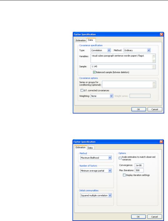
We illustrate the basic features of the factor object by analyzing a subset of the classic Holzinger and Swineford (1939) data, consisting of measures on 24 psychological tests for 145 Chicago area children attending the Grant-White school (Gorsuch, 1983). A large number of authors have used these data for illustrating various features of factor analysis. The raw data are provided in the EViews workfile “Holzinger24.WF1”. We will work with a subset consisting of seven of the 24 variables: VISUAL (visual perception), CUBES (spatial relations), PARAGRAPH (paragraph comprehension), SENTENCE (sentence completion), WORDM (word meaning), PAPER1 (paper shapes), and FLAGS1 (lozenge shapes).

(As noted by Gorsuch (1983, p. 12), the raw data and the published correlations do not match; for example, the data in “Holzinger24.WF1” produces correlations that differ from those reported in Table 7.4 of Harman (1976). Here, we will assume that the raw data are

An Example—723

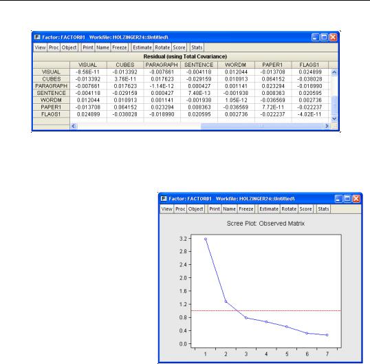
starting values for the communalities will be taken from the squared multiple correlations (SMCs). We will use the default settings for our example so you may click on OK to continue.

EViews estimates the model and displays the results view. Here, we see the top portion of the main results. The heading information provides basic information about the settings used in estimation, and basic status information. We see that the estimation used all 145 observations in the workfile, and converged after five iterations.

Factor Method: Maximum Likelihood

Date: 09/11/06 Time: 12:00

Covariance Analysis: Ordinary Correlation

Sample: 1 145

Included observations: 145

Number of factors: Minimum average partial

Prior communalities: Squared multiple correlation

Convergence achieved after 5 iterations

Below the heading is a section displaying the estimates of the unrotated orthogonal loadings, communalities, and uniqueness estimates obtained from estimation.

We first see that Velicer’s MAP method has retained two factors, labeled “F1” and “F2”. A brief examination of the unrotated loadings indicates that PARAGRAPH, SENTENCE and WORDM load on the first factor, while VISUAL, CUES, PAPER1, and FLAGS1 load on the second factor. We therefore might reasonably label the first factor as a measure of verbal ability and the second factor as an indicator of spatial ability. We will return to this interpretation shortly.

To the right of the loadings are communality and uniqueness estimates which apportion the diagonals of the correlation matrix into common (explained) and individual (unexplained) components. The communalities are obtained by computing the row norms of the loadings

matrix, while the uniquenesses are obtained directly from the ML estimation algorithm. We see, for example, that 56% (0.563 = 0.4912 + 0.5682 ) of the correlation for the VISUAL variable and 69% (0.692 = 0.8172 + (–0.155)2 ) of the SENTENCE correlation are

accounted for by the two common factors.

An Example—725

Goodness-of-fit Summary

Factor: FACTOR01

Date: 09/13/06 Time: 15:36

As you can see, EViews computes a large number of absolute and relative fit measures. In addition to the discrepancy, chi-square and Bartlett chi-square statistics seen previously, EViews computes scaled information criteria, expected cross-validation indices, generalized fit indices, as well as various measures based on estimates of noncentrality. Also presented are incremental fit indices which compare the fit of the estimated model against the independence model (see “Model Evaluation,” beginning on page 741 for discussion).

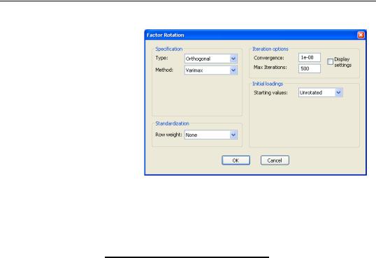
In addition, you may examine various matrices associated with the estimation procedure. You may examine the computed correlation matrix, various reduced and fitted matrices, and a variety of residual matrices. For example, you may view the residual variance matrix by selecting View/Residual Covariance Matrix/Using Total Covariance.

An Example—727

Kaiser's Measure of Sampling Adequacy

Factor: Untitled

Date: 09/12/06 Time: 10:04

The bottom portion of the display shows the matrix of partial correlations:

Each cell of this matrix contains the partial correlation for the two variables, controlling for the remaining variables.

Factor Rotation

Factor rotation may be used to simplify the factor structure and to ease the interpretation of factors. For this example, we will consider one orthogonal and one oblique rotation. To perform a factor rotation, click on the Rotate button on the factor toolbar or select Proc/ Rotate... from the main factor menu.

An Example—729

Note that the factor rotation and loading rotation matrices are identical since we are performing an orthogonal rotation.

Perhaps more interesting are the results for an oblique rotation. To replace the Varimax results with an oblique Quartimax/Quartimin rotation, select Proc/ Rotate... and change the

Type combo to Oblique, and select Quartimax. We will make a few other changes in the dialog. We will use random orthogonal rotations as starting values for our rotation, so that

under Starting values, you should select Random. Set the random generator options as depicted and change the convergence tolerance to 1e-06. By default, EViews will perform 25 oblique rotations using random orthogonal rotation matrices as the starting values, and will select the results with the smallest objective function value. Click on OK to accept these settings.

The top portion of the results shows information on the rotation method and initial loadings. Just below the header are the rotated loadings. Note that the relative importance of the VISUAL, CUBES, PAPER1, and FLAGS1 loadings on the second factor is somewhat more apparent for the oblique factors.

An Example—731

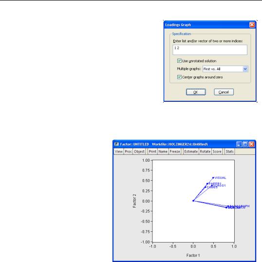
Once a rotation has been performed, the last set of rotated loadings will be available to all routines that use loadings. For example, to visualize the factor loadings, select View/Loadings/Loadings Graph...

to bring up the loadings graph dialog.

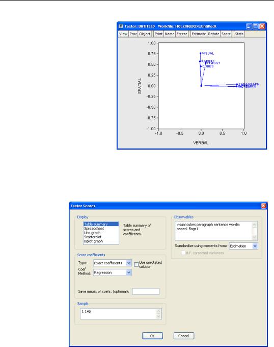
Here you will provide indices for the factor loadings you wish to display. Since there are only two factors, EViews has prefilled the dialog with “1 2” indicating that it will plot the second factor against the first factor.

By default, EViews will use the rotated loadings if available; note the checkbox allowing you to use the unrotated loadings. Check this box and click on OK to display the unrotated loadings graph.

As is customary, the loadings are displayed as lines from the origin to the points labeled with the variable name. Here we see visual evidence of our previous interpretation: the variables cluster naturally into two groups (factors), with factor 1 representing verbal ability (PARAGRAPH, SENTENCE, WORDM), and factor 2 representing spatial ability (VISUAL, PAPER1, FLAGS1, CUBES).

Before displaying the oblique Quartimax rotated loadings, we will apply this labeling to the

factors. Select Proc/Name Factors... and enter “Verbal” and “Spatial” in the dialog. EViews will subsequently label the factors using the specified names instead of the generic labels “Factor 1” and “Factor 2.”

An Example—733

ting, and the method for computing coefficients. Selecting Table summary, EViews produces output describing the score coefficient estimation.

The top portion of the output summarizes the factor score coefficient estimation settings and displays the factor coefficients used in computing scores:

Factor Score Summary

Factor: Untitled

Date: 09/12/06 Time: 11:52

Exact scoring coefficients

Method: Regression (based on rotated loadings)

Standardize observables using moments from estimation

Sample: 1 145

Included observations: 145

We see that the VERBAL score for an individual is computed as a linear combination of the centered data for VISUAL, CUBES, etc., with weights given by the first column of coefficients (0.03, 0.01, etc.).

The next section contains the factor indeterminacy indices:

The indeterminacy indices show that the correlation between the estimated factors and the variables is high; the multiple correlation for the first factor well over 0.90, while the correlation for the second factor is around 0.85. The minimum correlation indices are also reasonable, suggesting that alternative factor score solutions are highly correlated. At a minimum, the correlation between two different measures of the SPATIAL factors will be nearly 0.50.

The following sections report the validity coefficients, the off-diagonal elements of the univocality matrix, and for comparison purposes, the theoretical factor correlation matrix and estimated scores correlation:

An Example—735

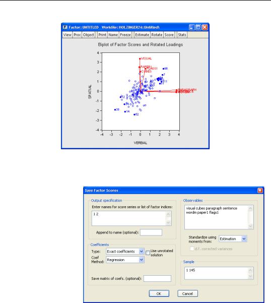
The positive correlation between the VERBAL and SPATIAL scores is obvious. The outliers show that individual 96 scores high and individual 38 low on both spatial and verbal ability, while individual 52 scores poorly on spatial relative to verbal ability.

To save scores to the workfile, select

Proc/Make Scores... and fill out the dialog. The procedure dialog differs from the view dialog only in the Output specification section. Here, you should enter a list of scores to be saved or a list of indices for the scores. Since we

have previously named our factors, we may specify the indices “1 2” and click on OK. EViews will open an untitled group containing the results saved in the series VERBAL and SPATIAL.