
- •Preface
- •Part IV. Basic Single Equation Analysis
- •Chapter 18. Basic Regression Analysis
- •Equation Objects
- •Specifying an Equation in EViews
- •Estimating an Equation in EViews
- •Equation Output
- •Working with Equations
- •Estimation Problems
- •References
- •Chapter 19. Additional Regression Tools
- •Special Equation Expressions
- •Robust Standard Errors
- •Weighted Least Squares
- •Nonlinear Least Squares
- •Stepwise Least Squares Regression
- •References
- •Chapter 20. Instrumental Variables and GMM
- •Background
- •Two-stage Least Squares
- •Nonlinear Two-stage Least Squares
- •Limited Information Maximum Likelihood and K-Class Estimation
- •Generalized Method of Moments
- •IV Diagnostics and Tests
- •References
- •Chapter 21. Time Series Regression
- •Serial Correlation Theory
- •Testing for Serial Correlation
- •Estimating AR Models
- •ARIMA Theory
- •Estimating ARIMA Models
- •ARMA Equation Diagnostics
- •References
- •Chapter 22. Forecasting from an Equation
- •Forecasting from Equations in EViews
- •An Illustration
- •Forecast Basics
- •Forecasts with Lagged Dependent Variables
- •Forecasting with ARMA Errors
- •Forecasting from Equations with Expressions
- •Forecasting with Nonlinear and PDL Specifications
- •References
- •Chapter 23. Specification and Diagnostic Tests
- •Background
- •Coefficient Diagnostics
- •Residual Diagnostics
- •Stability Diagnostics
- •Applications
- •References
- •Part V. Advanced Single Equation Analysis
- •Chapter 24. ARCH and GARCH Estimation
- •Basic ARCH Specifications
- •Estimating ARCH Models in EViews
- •Working with ARCH Models
- •Additional ARCH Models
- •Examples
- •References
- •Chapter 25. Cointegrating Regression
- •Background
- •Estimating a Cointegrating Regression
- •Testing for Cointegration
- •Working with an Equation
- •References
- •Binary Dependent Variable Models
- •Ordered Dependent Variable Models
- •Censored Regression Models
- •Truncated Regression Models
- •Count Models
- •Technical Notes
- •References
- •Chapter 27. Generalized Linear Models
- •Overview
- •How to Estimate a GLM in EViews
- •Examples
- •Working with a GLM Equation
- •Technical Details
- •References
- •Chapter 28. Quantile Regression
- •Estimating Quantile Regression in EViews
- •Views and Procedures
- •Background
- •References
- •Chapter 29. The Log Likelihood (LogL) Object
- •Overview
- •Specification
- •Estimation
- •LogL Views
- •LogL Procs
- •Troubleshooting
- •Limitations
- •Examples
- •References
- •Part VI. Advanced Univariate Analysis
- •Chapter 30. Univariate Time Series Analysis
- •Unit Root Testing
- •Panel Unit Root Test
- •Variance Ratio Test
- •BDS Independence Test
- •References
- •Part VII. Multiple Equation Analysis
- •Chapter 31. System Estimation
- •Background
- •System Estimation Methods
- •How to Create and Specify a System
- •Working With Systems
- •Technical Discussion
- •References
- •Vector Autoregressions (VARs)
- •Estimating a VAR in EViews
- •VAR Estimation Output
- •Views and Procs of a VAR
- •Structural (Identified) VARs
- •Vector Error Correction (VEC) Models
- •A Note on Version Compatibility
- •References
- •Chapter 33. State Space Models and the Kalman Filter
- •Background
- •Specifying a State Space Model in EViews
- •Working with the State Space
- •Converting from Version 3 Sspace
- •Technical Discussion
- •References
- •Chapter 34. Models
- •Overview
- •An Example Model
- •Building a Model
- •Working with the Model Structure
- •Specifying Scenarios
- •Using Add Factors
- •Solving the Model
- •Working with the Model Data
- •References
- •Part VIII. Panel and Pooled Data
- •Chapter 35. Pooled Time Series, Cross-Section Data
- •The Pool Workfile
- •The Pool Object
- •Pooled Data
- •Setting up a Pool Workfile
- •Working with Pooled Data
- •Pooled Estimation
- •References
- •Chapter 36. Working with Panel Data
- •Structuring a Panel Workfile
- •Panel Workfile Display
- •Panel Workfile Information
- •Working with Panel Data
- •Basic Panel Analysis
- •References
- •Chapter 37. Panel Estimation
- •Estimating a Panel Equation
- •Panel Estimation Examples
- •Panel Equation Testing
- •Estimation Background
- •References
- •Part IX. Advanced Multivariate Analysis
- •Chapter 38. Cointegration Testing
- •Johansen Cointegration Test
- •Single-Equation Cointegration Tests
- •Panel Cointegration Testing
- •References
- •Chapter 39. Factor Analysis
- •Creating a Factor Object
- •Rotating Factors
- •Estimating Scores
- •Factor Views
- •Factor Procedures
- •Factor Data Members
- •An Example
- •Background
- •References
- •Appendix B. Estimation and Solution Options
- •Setting Estimation Options
- •Optimization Algorithms
- •Nonlinear Equation Solution Methods
- •References
- •Appendix C. Gradients and Derivatives
- •Gradients
- •Derivatives
- •References
- •Appendix D. Information Criteria
- •Definitions
- •Using Information Criteria as a Guide to Model Selection
- •References
- •Appendix E. Long-run Covariance Estimation
- •Technical Discussion
- •Kernel Function Properties
- •References
- •Index
- •Symbols
- •Numerics

716—Chapter 39. Factor Analysis
cipal components (see “Other Graphs (Variable Loadings, Component Scores, Biplots),” beginning on page 414).
Saving Scores
The score procedure allows you to save score values to series in the workfile. When saving scores using the Proc/Make Scores..., EViews opens a dialog that differs only slightly from the view dialog. Instead of a Display section, EViews provides an Output specification section in which you should enter a list of scores to be saved or a list of indices for the scores in the edit field.
To save the first two factors as series AA and BB, you may enter “AA BB” in the edit field. If, instead, you provide the indices “1 2”, EViews will save the first two factors using the default names “F1” and “F2”, unless you have previously named your factors using Proc/ Name Factors....
Factor Views
EViews provides a number of factor object views that allow you to examine the properties of your estimated factor model.
Specification
The specification view provides a text representation of the estimation specification, as well as the rotation specifications and assigned factor names (if relevant).
In this example, we see that we have estimated a ML factor model for seven variables, using a convergence criterion of 1e-07. The model was estimated using the default SMCs initial communalities and Velicer’s
MAP criterion to select the number of factors.
In addition, the object has a valid rotation method, oblique Quartimax, that was estimated using the default 25 random oblique rotations. If no rotations had been performed, the rotation specification would have read “Factor does not have a valid rotation.”
Lastly, we see that we have provided two factor names, “Verbal”, and “Spatial”, that will be used in place of the default names of the first two factors “F1” and “F2”.

Factor Views—717
Estimation Output
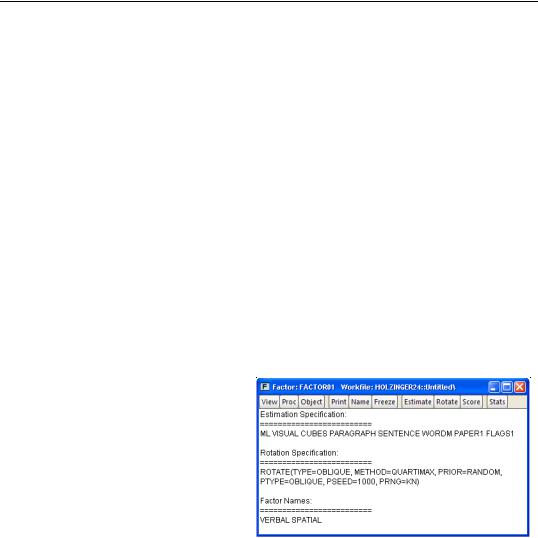
Select View/Estimation Output to display the main estimation output (unrotated loadings, communalities, uniquenesses, variance accounted for by factors, selected goodness-of-fit statistics). Alternately, you may click on the Stats toolbar button to display this view.
Rotation Results
Click View/Rotation Results to show the output table produced when performing a rotation (rotated loadings, factor correlation, factor rotation matrix, loading rotation matrix, and rotation objective function values).
Goodness-of-fit Summary
Select View/Goodness-of-fit Summary to display a table of goodness-of-fit statistics. For models estimated by ML or GLS, EViews computes a large number of absolute and relative fit measures. For details on these measures, see “Model Evaluation,” beginning on
page 741.
Matrix Views
You may display spreadsheet views of various matrices of interest. These matrix views are divided into four groups: matrices based on the observed dispersion matrix, matrices based on the reduced matrix, fitted matrices, and residual matrices.
Observed Covariances
You may examine the observed matrices by selecting View/Observed Covariance Matrix/ and the desired sub-matrix:
•The Covariance entry displays the original dispersion matrix, while the Scaled Covariance matrix scales the original matrix to have unit diagonals. In the case where the original matrix is a correlation, these two matrices will obviously be the same.
•Observations displays a matrix of the number of observations used in each pairwise comparison.
•If you select Anti-image Covariance, EViews will display the anti-image covariance of the original matrix. The anti-image covariance is computed by scaling the rows and columns of the inverse (or generalized inverse) of the original matrix by the inverse of its diagonals:
A= diag(S–1)–1S–1diag(S–1)–1
•Partial correlations will display the matrix of partial correlations, where every element represents the partial correlation of the variables conditional on the remaining variables. The partial correlations may be computed by scaling the anti-image covariance to unit diagonals and then performing a sign adjustment.

718—Chapter 39. Factor Analysis
Reduced Covariance
You may display the initial or final reduced matrices by selecting View/Reduced Covariance Matrix/ and Using Initial Uniqueness or Using Final Uniqueness.
Fitted Covariances
To display the fitted covariance matrices, select View/Fitted Covariance Matrix/ and the desired sub-matrix. Total Covariance displays the estimated covariance using both the common and unique variance estimates, while Common Covariance displays the estimate of the variance based solely on the common factors.
Residual Covariances
The different residual matrices are based on the total and the common covariance matrix. Select View/Residual Covariance Matrix/ and the desired matrix, Using Total Covariance, or Using Common Covariance. The residual matrix computed using the total covariance will generally have numbers close to zero on the main diagonal; the matrix computed using the common covariance will have numbers close to the uniquenesses on the diagonal (see “Scaling,” on page 711 for caveats).
Factor Structure Matrix
The factor structure matrix reports the correlations between the variables and factors. The correlation is equal to the (possibly rotated) loadings matrix times the factor correlation matrix, LF ; for orthogonal factors, the structure matrix simplifies so that the correlation is given by the loadings matrix, L .
Loadings Views
You may examine your rotated or unrotated loadings in spreadsheet or graphical form.
You may View/Loadings/Loadings Matrix to display the current loadings matrix in spreadsheet form. If a rotation has been performed, then this view will show the rotated loadings, otherwise it will display the unrotated loadings. To view the unrotated loadings, you may always select View/Loadings/Unrotated Loadings Matrix.

Factor Views—719
To display the loadings as a graph, select View/ Loadings/Loadings Graph... The dialog will prompt you for a set of indices for the factors you wish to plot. EViews will produce pairwise plots of the factors, with the loadings displayed as lines from the origin to the points labeled with the variable name.
By default, EViews will use the rotated solution if available; to override this choice, click on the Use unrotated solution checkbox.
The other settings allow you to control the handling of multiple graphs, and whether the graphs should be centered around the origin.
Scores
Select View/Scores... to compute estimates of factor score coefficients and to compute factor score values for observations. This view and the corresponding procedure are described in detail in “Estimating Scores,” on page 713.
Eigenvalues
One important class of factor model diagnostics is an examination of eigenvalues of the unreduced and the reduced matrices. In addition to being of independent interest, these eigenvalues are central to various methods for selecting the number of factors.
Select View/Eigenvalues... to open the Eigenvalue Display dialog. By default, EViews will display a table view containing a description of the eigenvalues of the observed dispersion matrix.
The dialog options allow you to control the output format and method of calculation:
•You may change the Output format to display a graph of the ordered eigenvalues. By default, EViews will display the resulting Scree plot along with a line representing the mean eigenvalue.
•To base calculations on the scaled observed, initial reduced or final reduced matrix, select the appropriate item in the Eigenvalues of combo.
•For table display, you may include the corresponding eigenvectors and dispersion matrix in the output by clicking on the appropriate Additional output checkbox.