
- •Preface
- •Part IV. Basic Single Equation Analysis
- •Chapter 18. Basic Regression Analysis
- •Equation Objects
- •Specifying an Equation in EViews
- •Estimating an Equation in EViews
- •Equation Output
- •Working with Equations
- •Estimation Problems
- •References
- •Chapter 19. Additional Regression Tools
- •Special Equation Expressions
- •Robust Standard Errors
- •Weighted Least Squares
- •Nonlinear Least Squares
- •Stepwise Least Squares Regression
- •References
- •Chapter 20. Instrumental Variables and GMM
- •Background
- •Two-stage Least Squares
- •Nonlinear Two-stage Least Squares
- •Limited Information Maximum Likelihood and K-Class Estimation
- •Generalized Method of Moments
- •IV Diagnostics and Tests
- •References
- •Chapter 21. Time Series Regression
- •Serial Correlation Theory
- •Testing for Serial Correlation
- •Estimating AR Models
- •ARIMA Theory
- •Estimating ARIMA Models
- •ARMA Equation Diagnostics
- •References
- •Chapter 22. Forecasting from an Equation
- •Forecasting from Equations in EViews
- •An Illustration
- •Forecast Basics
- •Forecasts with Lagged Dependent Variables
- •Forecasting with ARMA Errors
- •Forecasting from Equations with Expressions
- •Forecasting with Nonlinear and PDL Specifications
- •References
- •Chapter 23. Specification and Diagnostic Tests
- •Background
- •Coefficient Diagnostics
- •Residual Diagnostics
- •Stability Diagnostics
- •Applications
- •References
- •Part V. Advanced Single Equation Analysis
- •Chapter 24. ARCH and GARCH Estimation
- •Basic ARCH Specifications
- •Estimating ARCH Models in EViews
- •Working with ARCH Models
- •Additional ARCH Models
- •Examples
- •References
- •Chapter 25. Cointegrating Regression
- •Background
- •Estimating a Cointegrating Regression
- •Testing for Cointegration
- •Working with an Equation
- •References
- •Binary Dependent Variable Models
- •Ordered Dependent Variable Models
- •Censored Regression Models
- •Truncated Regression Models
- •Count Models
- •Technical Notes
- •References
- •Chapter 27. Generalized Linear Models
- •Overview
- •How to Estimate a GLM in EViews
- •Examples
- •Working with a GLM Equation
- •Technical Details
- •References
- •Chapter 28. Quantile Regression
- •Estimating Quantile Regression in EViews
- •Views and Procedures
- •Background
- •References
- •Chapter 29. The Log Likelihood (LogL) Object
- •Overview
- •Specification
- •Estimation
- •LogL Views
- •LogL Procs
- •Troubleshooting
- •Limitations
- •Examples
- •References
- •Part VI. Advanced Univariate Analysis
- •Chapter 30. Univariate Time Series Analysis
- •Unit Root Testing
- •Panel Unit Root Test
- •Variance Ratio Test
- •BDS Independence Test
- •References
- •Part VII. Multiple Equation Analysis
- •Chapter 31. System Estimation
- •Background
- •System Estimation Methods
- •How to Create and Specify a System
- •Working With Systems
- •Technical Discussion
- •References
- •Vector Autoregressions (VARs)
- •Estimating a VAR in EViews
- •VAR Estimation Output
- •Views and Procs of a VAR
- •Structural (Identified) VARs
- •Vector Error Correction (VEC) Models
- •A Note on Version Compatibility
- •References
- •Chapter 33. State Space Models and the Kalman Filter
- •Background
- •Specifying a State Space Model in EViews
- •Working with the State Space
- •Converting from Version 3 Sspace
- •Technical Discussion
- •References
- •Chapter 34. Models
- •Overview
- •An Example Model
- •Building a Model
- •Working with the Model Structure
- •Specifying Scenarios
- •Using Add Factors
- •Solving the Model
- •Working with the Model Data
- •References
- •Part VIII. Panel and Pooled Data
- •Chapter 35. Pooled Time Series, Cross-Section Data
- •The Pool Workfile
- •The Pool Object
- •Pooled Data
- •Setting up a Pool Workfile
- •Working with Pooled Data
- •Pooled Estimation
- •References
- •Chapter 36. Working with Panel Data
- •Structuring a Panel Workfile
- •Panel Workfile Display
- •Panel Workfile Information
- •Working with Panel Data
- •Basic Panel Analysis
- •References
- •Chapter 37. Panel Estimation
- •Estimating a Panel Equation
- •Panel Estimation Examples
- •Panel Equation Testing
- •Estimation Background
- •References
- •Part IX. Advanced Multivariate Analysis
- •Chapter 38. Cointegration Testing
- •Johansen Cointegration Test
- •Single-Equation Cointegration Tests
- •Panel Cointegration Testing
- •References
- •Chapter 39. Factor Analysis
- •Creating a Factor Object
- •Rotating Factors
- •Estimating Scores
- •Factor Views
- •Factor Procedures
- •Factor Data Members
- •An Example
- •Background
- •References
- •Appendix B. Estimation and Solution Options
- •Setting Estimation Options
- •Optimization Algorithms
- •Nonlinear Equation Solution Methods
- •References
- •Appendix C. Gradients and Derivatives
- •Gradients
- •Derivatives
- •References
- •Appendix D. Information Criteria
- •Definitions
- •Using Information Criteria as a Guide to Model Selection
- •References
- •Appendix E. Long-run Covariance Estimation
- •Technical Discussion
- •Kernel Function Properties
- •References
- •Index
- •Symbols
- •Numerics

712—Chapter 39. Factor Analysis
Heywood Case Handling
In the course of iterating principal factor estimation, one may encounter estimated communalities which implies that at least one unique variance is less than zero; these situations are referred to as Heywood cases.
When you encounter a Heywood case in EViews, there are several approaches that you may take. By default, EViews will stop iterating and report the final set of estimates (Stop and report final), along with a warning that the results may be inappropriate. Alternately, you may instruct EViews to report the previous iteration’s results (Stop and report last), to set the results to zero and continue (Set to zero, continue), or to ignore the negative unique variance and continue (Ignore and continue).
Rotating Factors
You may perform factor rotation on an estimated factor object with two or more retained factors. Simply call up the Factor Rotation dialog by clicking on the Rotate button or by selecting Proc/Rotate... from the factor object menu, and select the desired rotation settings.
The Type and Method combos may be used to specify the basic rotation method (see “Types of Rotation,” on page 744 for a description of the supported methods). For some methods, you will also be prompted to enter parameter values.
In the depicted example, we specify an oblique Promax rotation with a power
parameter of 3.0. The Promax orthogonal pre-rotation step performs Varimax (Orthomax with a parameter of 1).
By default, EViews does not row weight the loadings prior to rotation. To standardize the data, simply change the Row weight combo box to Kaiser or Cureton-Mulaik.
In addition, EViews uses the identity matrix (unrotated loadings) as the default starting value for the rotation iterations. The section labeled Starting values allows you to perform different initializations:

Estimating Scores—713
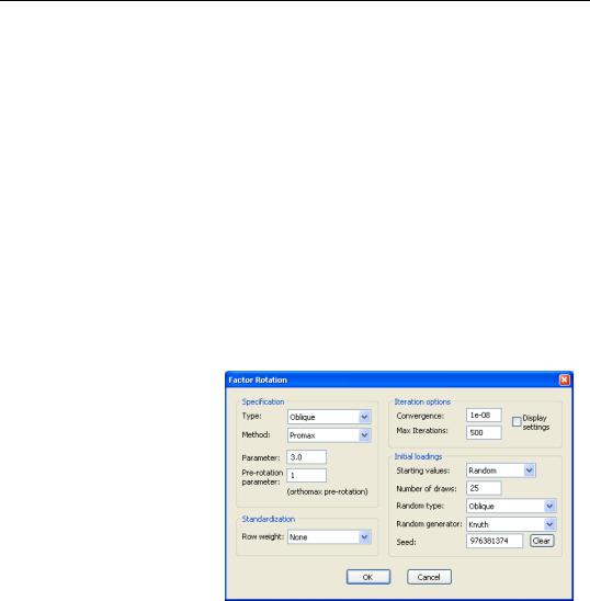
•You may instruct EViews to use an initial random rotation by selecting Random in the Starting values combo. The dialog changes to prompt you to specify the number of random starting matrices to compare, the random number generator, and the initial seed settings. If you select random, EViews will perform the requested number of rotations, and will use the rotation that minimizes the criterion function.
As with the random number generator used in parallel analysis, the value of this initial seed will be saved with the factor object so that by default, subsequent rotation will employ the same random values. You may override this initialization by entering a value in the Seed edit field or press the Clear button to have EViews draw a new random seed value.
•You may provide a user-specified initial rotation. Simply select User-specified in the Starting values combo, the provide the name of a m ¥ m matrix to be used as the starting T .
•Lastly, if you have previously performed a rotation, you may use the existing results as starting values for a new rotation. You may, for example, perform an oblique Quartimax rotation starting from an orthogonal Varimax solution.
Once you have specified your rotation method you may click on OK. EViews will estimate the rotation matrix, and will present a table reporting the rotated loadings, factor correlation, factor rotation matrix, loading rotation matrix, and rotation objective function values. Note that the factor structure matrix is not included in the table output; it may be viewed separately by selecting View/Structure Matrix from the factor object menu.
In addition EViews will save the results from the rotation with the factor object. Other routines that rely on estimated loadings such as factor scoring will offer you the option of using the unrotated or the rotated loadings. You may display your rotation results table at any time by selecting View/Rotation Results from the factor menu.
Estimating Scores
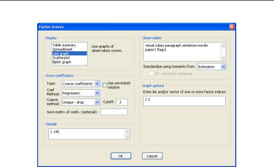
Factor score estimation may be performed as a factor object view or procedure.
Viewing Scores
To display score coefficients or scores, click on the Score button on the factor toolbar, or select View/Scores... from the factor menu.

714—Chapter 39. Factor Analysis
The scores view allows you to display: (1) a table showing the factor score coefficients, indeterminacy and validity indices, and univocality measures; (2) a table of factor score values for a set of observations; (3) a line graph of the scores; (4) scatterplots of scores on pairs of factors; (4) biplots of scores and loadings on pairs of factors.
You should specify the display format by clicking in the list box to choose one of: Table summary, Spreadsheet, Line graph, Scatterplot, and Biplot graph.
Scores Coefficients
To estimate scores, you must first specify a method for computing the score coefficients. For a brief discussion of methods, see “Score Estimation” on page 747. Details are provided in Gorsuch (1983), Ten Berge et. al (1999), Grice (2001), McDonald (1981), Green (1969).
You must first decide whether to use refined coefficients (Exact coefficients), to adjust the refined coefficients (Coarse coefficients), or to compute coarse coefficients based on the factor loadings (Coarse loadings). By default, EViews will compute scores estimates using exact coefficients.
Next, if rotated factors are available, they will be used as a default. You should check Use unrotated loadings to use the original loadings.
Depending on your selections, you will be prompted for additional information:
•If you select Exact coefficients or Coarse coefficients, EViews will prompt you for a Coef Method. You may choose between the following methods: Regression (Thurst-

Estimating Scores—715
one’s regression, Ideal variables (Harmon’s idealized variables), Bartlett WLS (Bartlett weighted least squares), Anderson-Rubin (Ten Berge et al. generalized Anderson-Rubin-McDonald), and Green (Green, MSE minimizing).
•If you select Coarse coefficients or Coarse loadings, EViews will prompt you for a coarse method and a cutoff value.
Simplified coefficient weights will be computed by recoding elements of the coefficient or loading matrix. In the Unrestricted method, values of the matrix that are greater (in absolute value) than some threshold are assigned sign-preserving values of -1 or 1; all other values are recoded at 0.
The two remaining methods restrict the coefficient weights so that each variable loads on a single factor. If you select Unique - recode, only the element with the highest absolute value in a row is recoded to a non-zero value; if you select Unique - drop, variables with more than loading in excess of the threshold are set to zero.
See Grice (2001) for discussion.
You may instruct EViews to save the matrix of scores coefficients in the workfile by entering a valid EViews object name in the Save matrix of coefs edit field.
Scores Data
You will need to specify a set of observable variables to use in scoring and a sample of observations. The estimated scores will be computed by taking linear combination of the standardized observables over the specified samples.
If available, EViews will fill the Observables edit field with the names of the original variables used in computation. You will be prompted for whether to standardize the specified data using the moments obtained from estimation, or whether to standardize the data using the newly computed moments obtained from the data. In the typical case, where we score observations using the same data that we used in estimation, these moments will coincide. When computing scores for observations or variables that differ from estimation, the choice is of considerable importance.
If you have estimated your object from a user-specified matrix, you must enter the names of the variables you wish to use as observables. Since moments of the original data are not available in this setting, they will be computed from the specified variables.
Graph Options
When displaying graph views of your results, you will be prompted for which factors to display; by default, EViews will graph all of your factors. Scatterplots and biplots provide additional options for handling multiple graphs, for centering the graph around 0, and for biplot graphs, labeling obs and loading scaling that should be familiar from our discussion of prin-