
- •Preface
- •Part IV. Basic Single Equation Analysis
- •Chapter 18. Basic Regression Analysis
- •Equation Objects
- •Specifying an Equation in EViews
- •Estimating an Equation in EViews
- •Equation Output
- •Working with Equations
- •Estimation Problems
- •References
- •Chapter 19. Additional Regression Tools
- •Special Equation Expressions
- •Robust Standard Errors
- •Weighted Least Squares
- •Nonlinear Least Squares
- •Stepwise Least Squares Regression
- •References
- •Chapter 20. Instrumental Variables and GMM
- •Background
- •Two-stage Least Squares
- •Nonlinear Two-stage Least Squares
- •Limited Information Maximum Likelihood and K-Class Estimation
- •Generalized Method of Moments
- •IV Diagnostics and Tests
- •References
- •Chapter 21. Time Series Regression
- •Serial Correlation Theory
- •Testing for Serial Correlation
- •Estimating AR Models
- •ARIMA Theory
- •Estimating ARIMA Models
- •ARMA Equation Diagnostics
- •References
- •Chapter 22. Forecasting from an Equation
- •Forecasting from Equations in EViews
- •An Illustration
- •Forecast Basics
- •Forecasts with Lagged Dependent Variables
- •Forecasting with ARMA Errors
- •Forecasting from Equations with Expressions
- •Forecasting with Nonlinear and PDL Specifications
- •References
- •Chapter 23. Specification and Diagnostic Tests
- •Background
- •Coefficient Diagnostics
- •Residual Diagnostics
- •Stability Diagnostics
- •Applications
- •References
- •Part V. Advanced Single Equation Analysis
- •Chapter 24. ARCH and GARCH Estimation
- •Basic ARCH Specifications
- •Estimating ARCH Models in EViews
- •Working with ARCH Models
- •Additional ARCH Models
- •Examples
- •References
- •Chapter 25. Cointegrating Regression
- •Background
- •Estimating a Cointegrating Regression
- •Testing for Cointegration
- •Working with an Equation
- •References
- •Binary Dependent Variable Models
- •Ordered Dependent Variable Models
- •Censored Regression Models
- •Truncated Regression Models
- •Count Models
- •Technical Notes
- •References
- •Chapter 27. Generalized Linear Models
- •Overview
- •How to Estimate a GLM in EViews
- •Examples
- •Working with a GLM Equation
- •Technical Details
- •References
- •Chapter 28. Quantile Regression
- •Estimating Quantile Regression in EViews
- •Views and Procedures
- •Background
- •References
- •Chapter 29. The Log Likelihood (LogL) Object
- •Overview
- •Specification
- •Estimation
- •LogL Views
- •LogL Procs
- •Troubleshooting
- •Limitations
- •Examples
- •References
- •Part VI. Advanced Univariate Analysis
- •Chapter 30. Univariate Time Series Analysis
- •Unit Root Testing
- •Panel Unit Root Test
- •Variance Ratio Test
- •BDS Independence Test
- •References
- •Part VII. Multiple Equation Analysis
- •Chapter 31. System Estimation
- •Background
- •System Estimation Methods
- •How to Create and Specify a System
- •Working With Systems
- •Technical Discussion
- •References
- •Vector Autoregressions (VARs)
- •Estimating a VAR in EViews
- •VAR Estimation Output
- •Views and Procs of a VAR
- •Structural (Identified) VARs
- •Vector Error Correction (VEC) Models
- •A Note on Version Compatibility
- •References
- •Chapter 33. State Space Models and the Kalman Filter
- •Background
- •Specifying a State Space Model in EViews
- •Working with the State Space
- •Converting from Version 3 Sspace
- •Technical Discussion
- •References
- •Chapter 34. Models
- •Overview
- •An Example Model
- •Building a Model
- •Working with the Model Structure
- •Specifying Scenarios
- •Using Add Factors
- •Solving the Model
- •Working with the Model Data
- •References
- •Part VIII. Panel and Pooled Data
- •Chapter 35. Pooled Time Series, Cross-Section Data
- •The Pool Workfile
- •The Pool Object
- •Pooled Data
- •Setting up a Pool Workfile
- •Working with Pooled Data
- •Pooled Estimation
- •References
- •Chapter 36. Working with Panel Data
- •Structuring a Panel Workfile
- •Panel Workfile Display
- •Panel Workfile Information
- •Working with Panel Data
- •Basic Panel Analysis
- •References
- •Chapter 37. Panel Estimation
- •Estimating a Panel Equation
- •Panel Estimation Examples
- •Panel Equation Testing
- •Estimation Background
- •References
- •Part IX. Advanced Multivariate Analysis
- •Chapter 38. Cointegration Testing
- •Johansen Cointegration Test
- •Single-Equation Cointegration Tests
- •Panel Cointegration Testing
- •References
- •Chapter 39. Factor Analysis
- •Creating a Factor Object
- •Rotating Factors
- •Estimating Scores
- •Factor Views
- •Factor Procedures
- •Factor Data Members
- •An Example
- •Background
- •References
- •Appendix B. Estimation and Solution Options
- •Setting Estimation Options
- •Optimization Algorithms
- •Nonlinear Equation Solution Methods
- •References
- •Appendix C. Gradients and Derivatives
- •Gradients
- •Derivatives
- •References
- •Appendix D. Information Criteria
- •Definitions
- •Using Information Criteria as a Guide to Model Selection
- •References
- •Appendix E. Long-run Covariance Estimation
- •Technical Discussion
- •Kernel Function Properties
- •References
- •Index
- •Symbols
- •Numerics

694—Chapter 38. Cointegration Testing
there is one cointegrating relation. Conditional on there being only one cointegrating relation, the LR test does not reject the imposed restriction at conventional levels.
The output also reports the estimated b and a imposing the restrictions. Since the cointegration test does not specify the number of cointegrating relations, results for all ranks that are consistent with the specified restrictions will be displayed. For example, suppose the restriction is:
B(2,1) = 1
Since this is a restriction on the second cointegrating vector, EViews will display results for ranks r = 2, 3, º, k – 1 (if the VAR has only k = 2 variables, EViews will return an error message pointing out that the “implied rank from restrictions must be of reduced order”).
For each rank, the output reports whether convergence was achieved and the number of iterations. The output also reports whether the restrictions identify all cointegrating parameters under the assumed rank. If the cointegrating vectors are identified, asymptotic standard errors will be reported together with the parameters b .
Single-Equation Cointegration Tests
You may use a group or an equation object estimated using cointreg to perform Engle and Granger (1987) or Phillips and Ouliaris (1990) single-equation residual-based cointegration tests. A description of the single-equation model underlying these tests is provided in “Background” on page 219. Details on the computation of the tests and the associated options may be found in “Residual-based Tests,” on page 234.
Briefly, the Engle-Granger and Phillips-Ouliaris residual-based tests for cointegration are simply unit root tests applied to the residuals obtained from a static OLS cointegrating regression. Under the assumption that the series are not cointegrated, the residuals are unit root nonstationary. Therefore, a test of the null hypothesis of no cointegration against the alternative of cointegration may be constructed by computing a unit root test of the null of residual nonstationarity against the alternative of residual stationarity.
How to Perform a Residual-Based Cointegration Test
We illustrate the single-equation cointegration tests using Hamilton’s (1994) purchasing power parity example (p. 598) for the log of the U.S. price level (P_T), log of the Dollar-Lira exchange rate (S_T), and the log of the Italian price level (PSTAR_T) from 1973m1 to 1989m10. We will use these data, which are provided in “Hamilton_rates.WF1”, to construct Engle-Granger and Phillips-Ouliaris tests assuming the constant is the only deterministic regressor in the cointegrating equation.
To carry out the Engle-Granger of Phillips-Ouliaris cointegration tests, first create a group, say G1, containing the series P_T, S_T, and PSTAR_T, then select View/Cointegration

Single-Equation Cointegration Tests—695
Test/Single-Equation Cointegration Test from the group toolbar or main menu. The Cointegration Test Specification page opens to prompt you for information about the test.
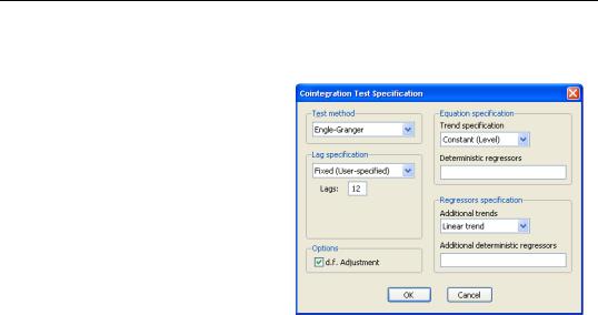
The combo box at the top allows you to choose between the default EngleGranger test or the Phillips-Ouliaris test. Below the combo are the options for the test statistic. The Engle-Granger test requires a specification for the number of lagged differences to include in the test regression, and whether to d.f. adjust the standard error estimate when forming the ADF test statistics. To match Hamilton’s example, we specify a Fixed (Userspecified) lag specification of 12, and retain the default d.f. correction of the standard error estimate.
The right-side of the dialog is used to specify the form of the cointegrating equation. The main cointegrating equation is described in the Equation specification section. You should use the Trend specification combo to choose from the list of pre-specified deterministic trend variable assumptions (None, Constant (Level), Linear Trend, Quadratic Trend). If you wish to include deterministic regressors that are not offered in the pre-specified list, you may enter the series names or expressions in the Deterministic regressors edit box. For our example, we will leave the settings at their default values, with the Trend specification set to Constant (Level), and no additional deterministic regressors specified.
The Regressors specification section should be used to specify any deterministic trends or other regressors that should be included in the regressors equations but not in the cointegrating equation. In our example, Hamilton points to evidence of non-zero drift in the regressors, so we will select Linear trend in the Additional trends combo.
Click on OK to compute and display the test results.

696—Chapter 38. Cointegration Testing
Date: 05/11/09 Time: 15:52
Series: P_T S_T PSTAR_T
Sample: 1973M01 1989M10
Included observations: 202
Null hypothesis: Series are not cointegrated
Cointegrating equation deterministics: C
Additional regressor deterministics: @TREND
Fixed lag specification (lag=12)
Dependent |
tau-statistic |
Prob.* |
z-statistic |
Prob.* |
P_T |
-2.730940 |
0.4021 |
-26.42791 |
0.0479 |
S_T |
-2.069678 |
0.7444 |
-13.83563 |
0.4088 |
PSTAR_T |
-2.631078 |
0.4548 |
-22.75737 |
0.0962 |
|
|
|
|
|
|
|
|
|
|
*MacKinnon (1996) p-values. |
|
|
|
|
Intermediate Results: |
|
|
|
|
|
|
P_T |
S_T |
PSTAR_T |
Rho - 1 |
|
-0.030478 |
-0.030082 |
-0.031846 |
Rho S.E. |
|
0.011160 |
0.014535 |
0.012104 |
Residual variance |
|
0.114656 |
5.934605 |
0.468376 |
Long-run residual variance |
2.413438 |
35.14397 |
6.695884 |
|
Number of lags |
|
12 |
12 |
12 |
Number of observations |
189 |
189 |
189 |
|
Number of stochastic trends** |
2 |
2 |
2 |
|
|
|
|
|
|
**Number of stochastic trends in asymptotic distribution
The top two portions of the output describe the test setup and summarize the test results. Regarding the test results, note that EViews computes both the Engle-Granger tau-statistic (t-statistic) and normalized autocorrelation coefficient (which we term the z-statistic) for residuals obtained using each series in the group as the dependent variable in a cointegrating regression. Here we see that the test results are broadly similar for different dependent variables, with the tau-statistic uniformly failing to reject the null of no cointegration at conventional levels. The results for the z-statistics are mixed, with the residuals from the P_T equation rejecting the unit root null at the 5% level. On balance, however, the test statistics suggest that we cannot reject the null hypothesis of no cointegration.
The bottom portion of the results show intermediate calculations for the test corresponding to each dependent variable. “Residual-based Tests,” on page 234 offers a discussion of these statistics. We do note that there are only 2 stochastic trends in the asymptotic distribution (instead of the 3 corresponding to the number of variables in the group) as a result of our assumption of a non-zero drift in the regressors.
Alternately, you may compute the Phillips-Ouliaris test statistic. Once again select View/ Cointegration Test/Single-Equation Cointegration Test from the Group toolbar or main menu, but this time choose Phillips-Ouliaris in the Test Method combo.

Single-Equation Cointegration Tests—697
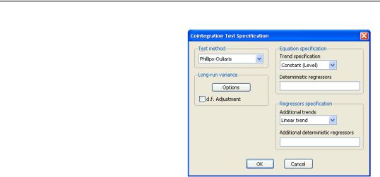
The right-hand side of the dialog, which describes the cointegrating regression and regressors specifications, should be specified as before.
The left-hand side of the dialog changes to show a single Options button for controlling the estimation of the Long-run variance used in the Phillips-Ouliaris test, and the checkbox for d.f Adjustment of the variance estimates. The default settings instruct EViews to compute these long-run variances using a non-prewhitened
Bartlett kernel estimator with a fixed Newey-West bandwidth. We match the Hamilton example settings by turning off the d.f. adjustment and by clicking on the Options button and using the Bandwidth method combo to specify a User-specified bandwidth value of 13.
Click on the OK button to accept the Options, then on OK again to compute the test statistics and display the results: