EViews Guides BITCH / EViews_tutorial

Estimating two-stage least squares regression using two distinct stages and OLS (UE, 14.3.1):

To estimate the two-stage least squares equation printed in UE, Equation 14.28, using ordinary OLS and two distinct phases, follow these steps:

Step 1. Open the EViews workfile named Macro14.wf1.

Step 2. To estimate the reduced form equation for YD (UE, Equation 14.27, p. 480), select Objects/New Object/Equation on the workfile menu bar, enter YD C G NX T CO(-1) R(-1) in the Equation Specification: window, and click OK.

Step 3. To generate the forecast values from this equation, select Forecast on the equation menu bar, enter YDF in the Forecast name: window, and click OK. EViews will create a new variable in the workfile named YDF.

Step 4. To estimate the second stage equation for CO (UE, Equation 14.29, p. 481), select Objects/New Object/Equation on the workfile menu bar, enter CO C YDF CO(-1) in the Equation Specification: window, and click OK. Note that we have used the instrumental variable YDF instead of the actual variable YD for disposable income. The method, dependent variable, and variable names are highlighted in yellow in the OLS regression output shown below.

Step 5. Select Name on the equation window menu bar, enter TSLS_OLS_CO in the Name to identify object: window, and. click OK.

Step 6. Select Save on the workfile menu bar to save your changes.

Dependent Variable: CO

Method: Least Squares

Date: 07/05/00 Time: 15:44

Sample(adjusted): 1964 1994

Included observations: 31 after adjusting endpoints

Comparing the OLS, EViews TSLS, and OLS two-stage models:

To compare the coefficients, std. Errors, and t-statistics for the three models discussed in this chapter, open the equations named OLS_CO, TSLS_CO and TSLS_OLS_CO, by double clicking their respective icons in the workfile window, and compare the regression output. To facilitate the process, the output for the OLS, EViews TSLS and OLS TSLS models are printed in this guide. Look at all three and compare the data printed in the red-boxed area for each regression. Note that the estimated coefficients are larger in the OLS_CO model compared to the TSLS_CO and TSLS_OLS_CO models. This supports the hypothesis that OLS estimates of coefficients have a positive bias in simultaneous equation models (simultaneity bias). Contrarily, TSLS estimated coefficients tend to have a downward bias. Note that the estimated coefficients are identical for the TSLS_CO and TSLS_OLS_CO models, but the standard errors (Std. Error in the EViews output) are smaller in the EViews TSLS estimated model, making the coefficients more significant (i.e., higher t-statistics). In order to get accurate estimates of standard errors and t- scores, the estimation should be done on a complete two-stage least squares program (like EViews TSLS). When OLS is used to estimate the second stage, it ignores the fact that the first stage was run at all (UE, footnote 11, p. 481).

The identification problem and the order condition (UE, 14.3.3):

In order to calculate two-stage least squares using the TSLS – Two-Stage Least Squares (TSNLS and ARMA) option, your specification must satisfy the order condition for identification, which states that there must be at least as many instruments as there are coefficients in your equation. The order condition for identification is easy to assess in EViews. Count, to make sure that the number of independent variables, not counting the constant, in the Equation Specification: window (i.e., YD & CO(-1) ) is less than or equal to the number of predetermined variables in the Instrument list: window (i.e., G, T, NX, CO(-1) & R(-1)). See graphic in the Two-stage least squares regression using EViews TSLS method section above.

Exercises:

9.Open EViews and open the EViews workfile named Macro14.wf1.

a.Refer to Estimating CO with least squares.

b.Refer to Step 2 of Estimating two-stage least squares regression using two distinct stages and OLS.

c.Refer to Steps 3 & 4 of Estimating two-stage least squares regression using two distinct stages and OLS.

d.Refer to Estimating two-stage least squares regression using EViews TSLS method.

12. Double click the icon in the EViews Macro14.wf1 workfile window to reactivate the UE, Equation 14.29. Click Estimate on the equation menu bar and click OK. The reason for this is to make sure that the residuals in the EViews workfile are from the TSLS_CO equation. If the icon is not in the workfile, you must go back and follow the steps outlined in Estimating two-stage least squares regression using EViews TSLS method.

a.Follow the procedures outlined in Chapter 9.

13.Open EViews and open the EViews workfile named Oats14.wf1.

d.Refer to Estimating CO with Least Squares (OLS) and Estimating two-stage least squares regression using EViews TSLS method.

e.Refer to Comparing the OLS, EViews TSLS, and OLS two-stage models.

Chapter 15: Forecasting

In this chapter:

1.Forecasting chicken consumption using OLS (UE 15.1, Equation 6.8, p. 501)

2.Forecasting chicken consumption using a generalized least squares (GLS) model estimated with the AR(1) method (UE 15.2.2)

3.Forecasting chicken consumption using a generalized least squares (GLS) model estimated with the Cochrane-Orcutt method (UE 15.2.2)

4.Forecasting confidence intervals (UE 15.2.3)

5.Forecasting with simultaneous equation systems (UE 15.2.4)

6.Forecasting with ARIMA models (UE 15.3)

7.Exercises

Forecasting chicken consumption using OLS (UE 15.1, Equation 6.8, p. 501):

The chicken demand model developed in Chapter 6 was estimated using data from 1951-1994. In order to forecast a variable beyond 1994, the workfile range and sample must be expanded. Follow these steps to forecast chicken consumption for 1995 - 1997 using ordinary least squares:

Step 1. Open the EViews workfile named Chick6.wf1.

Step 2. To expand the workfile range, select Procs/Change Workfile Range from the workfile menu bar, change the End date from 1994 to 1997, and click OK.

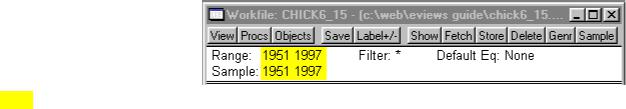
Step 3. To expand the sample, select Sample on the workfile menu bar, change the second number in the window from 1994 to 1997, and click OK. After Steps 2 & 3 are completed, the top portion of the EViews workfile should

look like the graphic on the right (note that the second date for Range: & Sample: have changed from 1994 to 1997).

Step 4. To open Y, PC, PB, & YD in a group window, hold down the Ctrl button, click on Y, PC, PB, & YD, select Show from the workfile toolbar, and click OK.

Step 5. To enter the data for Y, PC, PB, & YD from the text & footnote number 4 in UE, p. 502 (see table below), click edit+/- on the group menu bar, scroll to the bottom of the spreadsheet and replace the NA's with the appropriate numbers for the period 1995 - 1997. Press Enter after each entry and click edit+/- on the group menu bar a second time to save your changes. Scroll to the bottom of the group spreadsheet and make sure that it looks like the table below.

Forecasting chicken consumption using a generalized least squares model estimated with the Cochrane-Orcutt method(UE, 15.2.2):

The Cochrane-Orcutt method is a multi-step procedure that requires re-estimation until the value for the estimated first order serial correlation coefficient converges. Follow these steps to use the Cochrane-Orcutt method to estimate a GLS model for chicken consumption. If you have questions concerning the procedure, review the appropriate section of Chapter 9. Complete the section entitled Forecasting chicken consumption using OLS before attempting this section. The OLS estimate for chicken consumption should already have been estimated and saved as EQ01 in the Chick6.wf1 workfile and the workfile range & sample should have been expanded to 1997 and the data for 1995 - 1997 entered into the workfile spreadsheet.

Step 1. Open the EViews workfile named Chick6.wf1, select Sample on the workfile menu bar, change the End date from 1997 to 1994, and click OK.

Step 2. Open EQ01 by double clicking its icon in the workfile window. Create a new series for the residuals (errors) for EQ01, by selecting Procs/Make Residual Series on the EQ01 window menu bar, enter the name E as the Name for residual series, and click OK.

Step 3. Select Objects/New Object/Equation on the workfile menu bar. Enter E C E(-1) in the Equation Specification: window and click OK. The coefficient on the E(-1) term (i.e., ρ ), is positive and significant at the 1% level (t-statistic = 3.69 and Prob value = 0.0006). This evidence points to positive serial correlation. Select Name on the equation menu bar, enter EQ02 in the Name to identify object: window, and click OK.

Step 4. Select Objects/New Object/Equation on the workfile menu bar, enter Y- EQ02.@COEFS(2)*Y(-1) C PC-EQ02.@COEFS(2)*PC(-1) PB-EQ02.@COEFS(2)*PB(-1) YD- EQ02.@COEFS(2)*YD(-1) in the Equation Specification: window, and click OK. Select Name on the equation menu bar, enter EQ03 in the Name to identify object: window, and click OK.2

Step 5. Calculate the new residual series by typing the following formula in the command window: series E = Y-(EQ03.@COEFS(1) + EQ03.@COEFS(2)*PC + EQ03.@COEFS(3)*PB + EQ03.@COEFS(4)*YD) and pressing Enter on the keyboard.

Step 6. Re-run EQ02, EQ03 and the series E equation3 in step 5 sequentially until the estimated ρ (i.e., the coefficient on the E(-1) term from EQ02) does not change by more that a pre-selected value such as 0.001. After 6 iterations, the value for ρ converged (i.e., ρ changed from 0.902484 to 0.902802 between the 5th and 6th iteration).

Step 7. Convert the constant from the final version of EQ03 by typing the following formula in the command window: scalar beta0=EQ03.@COEFS(1)/(1-EQ02.@COEFS(2)) and pressing Enter on the keyboard.

Step 8. Double click the icon in the workfile window and read the value, 26.72580, for the estimated constant in the lower left of the screen. The final GLS equation for chicken consumption is Y = 26.72580 - 0.109891*PC + 0.090293*PB + 0.242032*YD, similar to the truncated coefficient model printed in UE, Equation 9.22, p. 507.

2Note that the variable names are truncated in the EViews regression output table because they don't fit in the variable name cell. Nonetheless, the regression is correct. The equation, with the entire variable names printed out, can be viewed by selecting View/Representations on the equation menu bar.

3You can re-run an equation by opening the equation in a window, selecting Estimate on the equation menu bar and clicking OK. You can re-run the series e equation by clicking the cursor anywhere on the equation in the command window and hitting Enter on the keyboard.

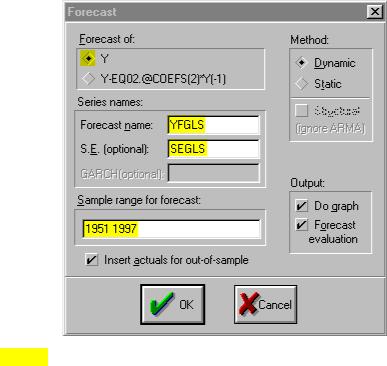
Step 9. Select Sample on the workfile menu bar and change the End date from 1994 to 1997. Open EQ03 and select Forecast on the equation menu bar. Make sure that Y is checked in the Forecast of: window. Change the Forecast name: to

YFGLS. Check to make sure that the Sample range to forecast: is set to 1951 1997, and click OK (see graphic on the right).

Step 10. Open YFGLS & Y in a group window by holding down the Ctrl button, clicking on YFGLS & Y, selecting Show from the workfile toolbar, and clicking OK. Scroll to the bottom of the group spreadsheet and make sure that it looks like the table below.

Step 11. Select Save on the workfile menu bar to save your changes.

Step 12. Note that the predicted values for YFGLS in the EViews spreadsheet are slightly different than those in the UE, p. 502 table. This is due to the fact that the text uses rounded coefficient values for Equation 9.22 and we used non-rounded EViews estimated values. Delete this group object when finished.

Forecasting confidence intervals (UE, 15.2.3):

Follow these steps to make a point prediction of the weight of a male who stands 6'1" tall and calculate the high and low estimated values for a 95% confidence interval.

Step 1. Open the EViews workfile named Htwt1.wf1.

Step 2. Follow Steps 2 & 3 of the section entitled Forecasting chicken consumption using OLS to expand the workfile range and sample range from 20 to 21. Double click the X variable icon in the workfile window, click edit+/- on the series menu bar, scroll to the bottom of the spreadsheet, replace the NA for the 21st observation with 13 (i.e., height in inches above 5'), and press Enter. To save your changes, click edit+/- on the series menu bar a second time.

Step 3. Select Objects/New Object/Equation on the workfile menu bar, enter Y C X in the Equation Specification: window, and click OK. Select Name on the equation menu bar and enter EQ01 in the Name to identify object: window.

Step 4. Select Forecast on the equation menu bar. Enter YF in the Forecast name: window. Check to make sure that the Sample range to forecast: is set to 1 21, and click OK. To view the forecast weight of the male student standing 6'1" tall, double click the YF series icon in the workfile window and scroll to the bottom. The forecast weight for the 21st observation is 186.2993.

Step 5. Select Sample on the workfile menu bar, change the Sample range pairs (or sample object to copy): to 1 20, and click OK.

Step 6. Select Procs/Make Residual Series on the EQ01 window menu bar. Enter the name E as the Name for residual series, and click OK.

Step 7. Generate a new series for the residuals squared (i.e., E2) by selecting Genr on the workfile menu bar, entering the equation: E2=E^2 in the Enter equation: window, and clicking OK.

Step 8. Generate a new series named XDEV2 for the residuals squared by selecting Genr on the workfile menu bar, entering the equation: XDEV2=(x-@mean(x))^2 in the Enter equation: window, and clicking OK.

Step 9. To calculate the upper confidence interval for the 6'1" student, type the following formula (all one equation) in the command window, and press Enter on the keyboard:

scalar YF_HIGH=Yf(21)+((@sum(E2)/@obs(E2)*(1+(1/@obs(E))+((X(21)- @mean(X))^2/@sum(XDEV2))))^.5)*@qtdist(.975,(eq01.@regobs-eq01.@ncoef))

Double click YF_HIGH in the workfile window to view the upper confidence interval in the lower left of the screen (i.e., ).

Step 10. To calculate the lower confidence interval for the 6'1"student, type the following formula (all one equation) in the command window and press Enter on the keyboard:

scalar YF_LOW=Yf(21)-((@sum(E2)/@obs(E2)*(1+(1/@obs(E))+((X(21)- @mean(X))^2/@sum(XDEV2))))^.5)*@qtdist(.975,(eq01.@regobs-eq01.@ncoef))

Double click YF_LOW in the workfile window to view the upper confidence interval in the lower left of the screen (i.e., )

Forecasting with simultaneous equation systems (UE 15.2.4):

EViews has a Type of Object: named Model that enables you to solve a system of simultaneous equations and use the model for forecasting and simulation. EViews models do not contain unknown coefficients to be estimated. Instead, the Model object allows you to solve for unknown values for the endogenous variables. For a description of various methods of creating model objects in EViews and techniques for using these objects to forecast and perform simulations see Help/Contents/Hypothesis Testing and Forecasting/Model Solve (Forecast and Simulation).

This topic is beyond the scope of this guide but, if you were to do it, you would follow these steps to forecast with a simultaneous equation model:

Step 1. Create a model by selecting Object/New Object/Model in the main toolbar, type in a name for your model in the Name for Object: window, click OK, and enter the previously estimated equations in the model window.

Step 2. To solve the model, simply select the Solve button in the model toolbar. You should see the Model Solution dialog box offering various options for controlling the solution process. EViews solves for the endogenous variables, given data for the exogenous variables.

Forecasting with ARIMA models (UE 15.3):

ARIMA (autoregressive, integrated, moving average) models use three tools for modeling the serial correlation in the disturbance:

1.The first tool is the autoregressive or AR term. The AR(1) model introduced above uses only the first-order term but, in general, you may use additional, higher-order AR terms. Each AR term corresponds to the use of a lagged value of the residual in the forecasting equation for the unconditional residual. An autoregressive model of order p is denoted as AR(p).

2.The second tool is the integration order term. Each integration order corresponds to differencing the series being forecast. A first-order integrated component means that the forecasting model is designed for the first difference of the original series. A second-order component corresponds to using second differences, and so on.

3.The third tool is the MA, or moving average term. A moving average forecasting model uses lagged values of the forecast error to improve the current forecast. A first-order moving average term uses the most recent forecast error, a second-order term uses the forecast error from the two most recent periods, and so on.

In ARIMA forecasting, you assemble a complete forecasting model by using combinations of the three building blocks described above. You can use the correlogram view of a series for this purpose (see Testing for nonstationarity by calculating the auto correlation function ACF for a description of this process).