EViews Guides BITCH / EViews_tutorial

Performing Granger Causality tests (UE 12.3):

To conduct Granger Causality test for CO and YD, follow these steps:

Step 1. Open the EViews workfile named Macro14.wf1.

Step 2. To Create an EViews group for the current purchases of goods and services (CO) and the level of disposable income (YD), hold down the Ctrl button, click on, CO and YD, select Show from the workfile toolbar, and click OK.

Step 3. Select Name on the Group Object menu bar, enter GROUP01 in the Name to identify object: window, and click OK.

Step 4. Select View/Granger Causality… on the Group Object menu bar. When you select the Granger Causality view, you will first see a dialog box asking for the number of lags to use in the test regressions. Change the number in the Lags to include: to 3 in the Lag Specification: window, and click OK.4 EViews returns the following pairwise Granger Causality Tests Table.

Pairwise Granger Causality Tests

Date: 07/01/00 Time: 14:43

Sample: 1963 1994

Lags: 3

Step 5. Based on the Probability values reported in the table, the hypothesis that YD does not Granger Cause CO cannot be rejected, but the hypothesis that CO does not Granger cause YD can be rejected. Therefore, it appears that Granger causality runs one way, from CO to YD, but not the other way.5

Testing for nonstationarity by calculating the auto correlation function ACF (UE 12.4.1, Equation 12.24, p. 425):

Follow these steps to calculate the auto correlation function ACF:

Step 1. Open the EViews workfile named Macro14.wf1.

Step 2. Open CO in one window by double clicking the series icon in the workfile window.

Step 3. To view the Autocorrelation and Partial Correlation, Select View/Correlogram…, on the CO series menu bar and a Correlogram Specification dialog box appears. Select level in the Correlogram of: window and enter 16 (the EViews default in this case) in the Lag Specification: lags to include: window, and click OK to reveal the EViews output below.

4In general, it is better to use more rather than fewer lags, since the theory is couched in terms of the relevance of all past information. You should pick a lag length that corresponds to reasonable beliefs about the longest time over which one of the variables could help predict the other.

5The reported F-statistics are the Wald statistics for the joint hypothesis that the coefficients on the lagged values of the other variable are zero for each equation (CO in the first equation and YD in the second equation for the table printed above). In case you want to determine significance by comparing the calculated F statistic with the critical F value from the F Table, the numerator degrees of freedom are given by the number of coefficient restrictions in the null hypothesis (i.e., the number of lags) and the denominator degrees of freedom are given by the total regression degrees of freedom.

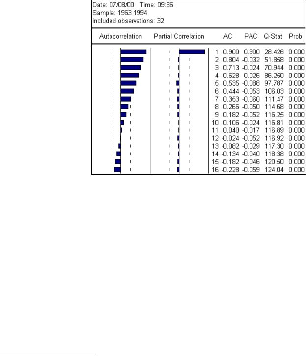
Step 4. Since the AC's are significantly positive and the AC(k) dies off geometrically with increasing lag k, it is a sign that the series obeys a low-order autoregressive (AR) process.6 In addition, since the partial autocorrelation (PAC) is significantly positive at lag 1 and close to zero thereafter, the pattern of autocorrelation can be captured by an autoregression of order one (i.e., AR(1)).

The finding in Steps 3 & 4 indicates that the CO

series violates the third criteria for stationarity (UE, top of p. 425) and provides strong evidence that the CO series is non-stationary.

Testing for nonstationarity with the Dickey-Fuller (DF) test (12.4.2):

Since the AC analysis in the previous section indicated that CO is most likely an AR(1) process, the Dickey-Fuller (DF) test is valid. Follow these steps to conduct the Dickey-Fuller test of the hypothesis that the CO series is non-stationary:

Step 1. Open the EViews workfile named Macro14.wf1.

Step 2. Open CO in one window by double clicking the series icon in the workfile window. Note that EViews will probably display the correlogram view for CO since that was the last view selected in the previous section. You can select View/Spreadsheet to view the series data or just proceed with the next step to test for stationarity.

Step 3. To conduct the Dickey-Fuller (DF) test, select View/Unit Root Test… on the CO series window menu bar.

Step 4. Four things have to be specified in the Unit Root Test dialog box to carry out a unit root test. First, choose the type of test—either the Augmented Dickey-Fuller (ADF) test or the Phillips-

6 If the AC(1) is nonzero, it means that the series is first order serially correlated. If AC(k) dies off more or less geometrically with increasing lag k, it is a sign that the series obeys a low-order autoregressive (AR) process. If AC(k) drops to zero after a small number of lags, it is a sign that the series obeys a low-order moving-average (MA) process. EViews also reports the Partial Correlations (PAC) in the same window. The partial correlation at lag k measures the correlation of CO values that are k periods apart, after removing the correlation from the intervening lags. If the pattern of autocorrelation is one that can be captured by an autoregression of order less than k, then the partial autocorrelation at lag k will be close to zero. The PAC of a pure autoregressive process of order k cuts off at lag k, while the PAC of a pure moving average (MA) process asymptotes gradually to zero.

Perron (PP) test (select ADF for this example).7 Second, specify whether to test for a unit root in the Level, 1st difference, or 2nd difference of the series (select level for this example).8 Third, specify whether to include an Intercept, a Trend and intercept, or None in the test regression. Select Trend and intercept for this example. To see why, read footnote 18, UE, p. 427. Fourth, specify the number of lagged first difference terms to add in the test regression (0 for the DF test). The theory behind each of these selections is beyond the scope of UE and this guide. Advanced econometrics courses deal with these issues. When finished with the selections click OK to reveal the following table:

Step 5. The test fails to reject the null hypothesis of a unit root in the CO series at any of the reported significance levels, since the ADF Test Statistic9 is not less than (i.e., does not lie to the left of) the MacKinnon critical values.

7EViews refers to both the Dickey-Fuller and the Augmented Dickey-Fuller tests as ADF tests. You will face two practical issues in performing the ADF test. First, you will have to specify the number of lagged first difference terms to add to the test regression (selecting zero yields the DF test; choosing numbers greater than zero generates ADF tests). The usual (though not particularly useful) advice is to include lags sufficient to remove any serial correlation in the residuals. Second, EViews asks you whether to include other exogenous variables in the test regression. You have the choice of including a constant, a constant and a linear time trend, or neither in the test regression.

8You can use this option to determine the number of unit roots in the series. If the test fails to reject the test in levels but rejects the test in first differences, then the series contains one unit root and is of integrated order one I(1). If the test fails to reject the test in levels and first differences but rejects the test in second differences, then the series contains two unit roots and is of integrated order two I(2).

9The output reports the ADF Test Statistic, but in reality, it is the DF test statistic, since zero lags were chosen.

Chapter 13: Dummy Dependent Variable Techniques

In this chapter:

1.Estimating the linear probability model (UE 13.1.3)

2.Estimating the Weighted Least Squares (WLS) correction for heteroskedasticity in the linear probability model (UE 13.1.3, pp. 441-442)

3.Estimating the binomial logit model (UE 13.2)

4.Estimating the binomial probit model (UE 13.3.1)

5.Interpreting the results of binary dependent variable regression

6.Estimating the multinomial logit model (UE 13.3.2)

7.Exercises

The workfile named women13.wf1 will be used to demonstrate the procedures explained in UE, Chapter 13. The data for this example are printed in UE, Table 13.1, p. 440. The name of the dummy variable is changed from D, in UE, Table 13.1, to j in the Women13.wf1 workfile (D is a reserved name in EViews).

Estimating the linear probability model (UE 13.1.3):

To estimate the linear probability model printed in UE, Equation 13.6, follow these steps:

Step 1. Open the EViews workfile named Women13.wf1.

Step 2. Select Objects/New Object/Equation on the workfile menu bar, enter J C M S in the Equation Specification: window, and click OK.

Step 3. Select Name on the equation menu bar, enter EQ01 in the Name to identify object: window, and click OK.

Step 4. Select Forecast on the equation menu bar, enter JFOLS in the Forecast name: window, and click OK.

Step 5. Enter the formula series JFOLSP = JFOLS >= 0.5 in the command window and press Enter. A series named JFOLSP is created that predicts whether a women is expected to be in the labor force based on the linear probability model. The formula applies the decision rule: JFOLSP is 1 if, the probability value, JFOLSi ≥ 0.5 and JFOLSP is 0 if JFOLSi < 0.5.

Step 6. Enter the formula series OLSP = JFOLSP=J in the command window and press Enter to calculate a series that equals 1 if the OLS model predicted correctly and 0 if not.

Step 7. Enter the formula scalar R2pOLS = @sum(OLSP)/@obs(OLSP) in the command window and press Enter to calculate the R2p value for the OLS model. Double click the icon to reveal the percentage of correct predictions from the OLS model on the status line in the lower left of the screen (0.8 for this exercise).

Step 8. Select Save on the workfile menu bar to save your changes.

Estimating the Weighted Least Squares (WLS) correction for heteroskedasticity in the linear probability model (UE 13.1.3, pp. 441-442):

To estimate the weighted least squares model specified in UE, Equations 13.7 & 13.8, follow these steps:

Step 1. Open the EViews workfile named women13.wf1.

Step 2. Select Objects/New Object/Equation on the workfile menu bar, enter J/Z C 1/Z M/Z S/Z in the Equation Specification: window, and click OK to generate the same coefficients and standard errors reported in UE, Equation 13.8.

Step 3. Select Name on the equation menu bar, enter EQ02a in the Name to identify object: window, and click OK.

Step 4. To perform the same analysis using the WLS feature in EViews: select Objects/New Object/Equation on the workfile menu bar, enter J Z C M S in the Equation Specification:

window, select the OOptions button, check Weighted LS/TSLS and type 1/Z in the Weight:

window. Click OK twice to generate the same coefficients and standard errors reported in UE, Equation 13.8. Note that the coefficient on the Z variable is the constant (i.e., Z*(1/Z) = 1) and the coefficient on the constant, C, is the coefficient on the variable 1/Z (i.e., C*(1/Z)).

Step 5. Select Name on the equation menu bar, enter EQ02b in the Name to identify object: window, and click OK.

Step 6. Select Forecast on the equation menu bar, enter JFWLS in the Forecast name: window, and click OK.

Step 7. Enter the formula series JFWLSP = JFWLS >= 0.5 in the command window and press Enter. A series named JFWLSP is created that predicts whether a women is expected to be in the labor force based on the linear probability model. The formula applies the decision rule: JFWLSP is 1 if, the probability value, JFWLSi ≥ 0.5 and JFWLSP is 0 if JFWLSi < 0.5.

Step 8. Enter the formula series WLSP =JFWLSP=J in the command window and press Enter to calculate a series that equals 1 if the WLS model predicted correctly and 0 if not.

Step 9. Enter the formula scalar R2pWLS = @sum(WLSP)/@obs(WLSP) in the command window and press Enter to calculate the R2p value for the WLS model. Double click the R2pWLS icon to reveal the percentage of correct predictions from the WLS model (0.83 for this exercise).

Step 10. Select Save on the workfile menu bar to save your changes.

Estimating the binomial logit model (UE 13.2):

To estimate the binomial logit model printed in UE, Equation 13.15, follow these steps:

Step 1. Open the EViews workfile named women13.wf1.

Step 2. Select Objects/New Object/Equation on the workfile menu bar.

Step 3. From the Estimation Settings:, Method: window, select the BINARY - Binary choice (logit, probit, extreme value…) estimation method. The window will change to reflect your choice.

Step 4. There are two parts to the binary model specification. First, in the Equation Specification: field, you should type the name of the Binary dependent variable followed by a list of regressors (i.e., enter J C M S in the Equation Specification: window for this example). Second, check logit as the Binary estimation method: (this is the default setting in EViews). Click OK to run the logit regression.

Step 5. Select Name on the equation menu bar, enter EQ03 in the Name to identify object: window, and click OK.

Step 6. Select Forecast on the equation menu bar, enter JFLOG in the Forecast name: window, and click OK.

Step 7. Enter the formula series JFLOGP = JFLOG >= 0.5 in the command window and press Enter. A series named JFLOGP is created that predicts whether a women is expected to be in the labor force based on the linear probability model. The formula applies the decision rule: JFLOGP is 1 if, the probability value, JFLOGi ≥ 0.5 and JFLOGP is 0 if JFLOGi < 0.5.

Step 8. Enter the formula series LOGP = JFLOGP=J in the command window and press Enter to calculate a series that equals 1 if the LOG model predicted correctly and 0 if not.

Step 9. Enter the formula scalar R2pLOG = @sum(LOGP)/@obs(LOGP) in the command window and press Enter to calculate the R2p value for the LOG model. Double click the R2pLOG icon to reveal the percentage of correct predictions from the LOG model (0.8 for this exercise).

Step 10. Select Save on the workfile menu bar to save your changes.

The linear probability model results and the binomial logit model results can be compared by opening both regression equation results in the work area (i.e., double click the EQ01 and EQ03 equation icons in the workfile window.

Estimating the binomial probit model (UE 13.3.1):

To estimate the binomial probit model printed in UE, Equation 13.19, follow these steps:

Step 1. Open the EViews workfile named women13.wf1.

Step 2. Select Objects/New Object/Equation on the workfile menu bar.

Step 3. From the Equation Specification: window, select the BINARY - Binary choice (logit, probit, extreme value…) estimation method. The window will change to reflect your choice.

Step 4. There are two parts to the binary model specification. First, in the Equation Specification: field, you should type the name of the Binary dependent variable followed by a list of regressors (i.e., enter J C M S in the Equation Specification: window for this example). Second, check probit as the Binary estimation method: (logit is the default setting in EViews). Click OK to run the probit regression.

Step 5. Select Name on the equation menu bar, enterEQ04 in the Name to identify object: window, and click OK.

Step 6. Select Forecast on the equation menu bar, enter JFPRO in the Forecast name: window, and click OK.

Step 7. Enter the formula series JFPROP = JFPRO >= 0.5 in the command window and press Enter. A series named JFPROP is created that predicts whether a women is expected to be in the labor force based on the linear probability model. The formula applies the decision rule: JFPROP is 1 if, the probability value, JFPROi ≥ 0.5 and JFPROP is 0 if JFPROi < 0.5.

Step 8. Enter the formula series PROP = JFPROP=J to calculate a series that equals 1 if the PRO model predicted correctly and 0 if not.

Step 9. Enter the formula scalar R2pPRO = @sum(PROP)/@obs(PROP) to calculate the R2p value for the PRO model. Double click the R2pPRO icon to reveal the percentage of correct predictions from the PRO model (0.8 for this exercise).

Step 10. Select Save on the workfile menu bar to save your changes.

Interpreting the results of binary dependent variable regression:

The estimated coefficient on each independent variable is easy to interpret in an OLS model, but difficult to interpret in a model estimated using the probit or logit technique. However, the relative size of each coefficient reflects the relative effect of the independent variables on the predicted probability for the dependent variable. Interpretation of the coefficient values is complicated by the fact that estimated coefficients from a binary dependent model cannot be interpreted as the marginal effect on the dependent variable.

Estimating the multinomial logit model (UE 13.3.2):

The multinomial logit process will not be discussed in detail here because the EViews 3.1 Student Version does not have the capability of estimating such programs.

Exercises:

8.

a.

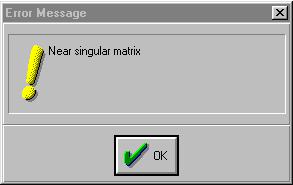
b.EViews gives you the error message Near singular matrix when the logit is used to estimate the model with the Equation Specification: J C M S AD (see graphic on the right.

9.Follow the procedures outlined in:

a.Estimating the linear probability model.

b.Estimating the binomial logit model.

c.Estimating the binomial probit model.

12.Open the EViews workfile named Mort13.wf1.

b.See Estimating the linear probability model.

c.See Estimating the linear probability model.

d.

e. See Estimating the linear probability model and Estimating the binomial logit model.

Chapter 14: Simultaneous Equations

In this chapter:

1.Generating time series for taxes and net exports using structural equations (UE, p. 477)

2.Estimating CO with least squares (UE, Equation 14.31, p. 481)

3.Estimating two-stage least squares regression using EViews TSLS method (UE, 14.3.3)

4.Estimating two-stage least squares regression using two distinct stages and OLS (UE, 14.3.1)

5.Comparing the OLS, EViews TSLS, and OLS two-stage models

6.The identification problem and the order condition (UE, 14.3.3)

7.Exercises

The naïve Keynesian macroeconomic model of the U.S. economy identified in UE, p. 477 will be used to demonstrate the two stage-least squares procedure. The data for this model is found in the EViews workfile named macro14.wf1 and it is printed in UE, Table 14.1, p. 478. Two variables that are included in the macroeconomic model must be generated from other data series (see note at the bottom of UE, Table 14.1, p. 478).

Generating time series for taxes and net exports using structural equations (UE, p. 477):

Follow these steps to generate time series values for T (taxes) and NX (net exports) using the structural equations in the model:

Step 1. Open the EViews workfile named Macro14.wf1.

Step 2. To generate a new series named T for taxes, select Genr on the workfile menu bar, type T=Y- YD in the Enter equation: window, and click OK. A new series icon for T is created in the workfile window.

Step 3. To generate a new series named NX for net exports, select Genr on the workfile menu bar, type NX=Y-CO-I-G in the Enter equation: window, and click OK. A new series icon for NX is created in the workfile window.

Step 4. Select Save on the workfile menu bar to save your changes.

Estimating CO with least squares (UE, Equation 14.31, p. 481):

Step 1. Open the EViews workfile named Macro14.wf1.

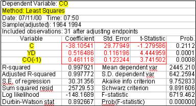
Step 2. Select Objects/New Object/Equation on the workfile menu bar, enter CO C YD CO(-1) in the Equation Specification: window, and click OK to reveal the regression output to the right.

Step 3. Select Name on the equation window menu bar, enter OLS_CO in the Name to identify object: window, and click OK.

Step 4. Select Save on the workfile menu bar to save your changes.

Estimating two-stage least squares regression using EViews TSLS method (UE, 14.3.1):

To estimate the two-stage least squares model printed in UE, Equation 14.29, follow these steps:

Step 1. Open the EViews workfile named

Macro14.wf1.

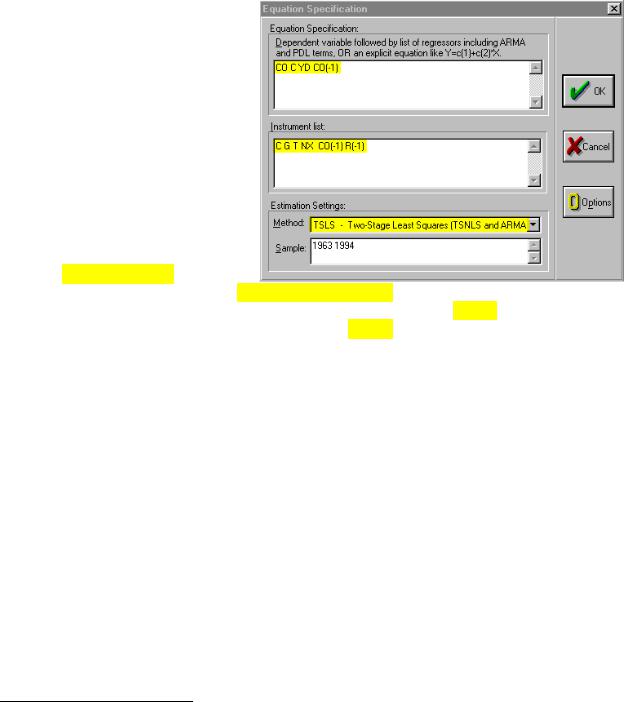
Step 2. Select Objects/New Object/Equation on the workfile menu bar, and select TSLS – Two-Stage Least Squares (TSNLS and ARMA) in the Method: window under Estimation Settings: and the dialog will change to include an Instrument list: window (see graphic on the right).

Step 3. Enter CO C YD CO(-1) in the

Equation Specification: window and C G T NX CO(-1) R(-1) in the Instrument list: window.1 The graphic above shows the relevant selections/entries highlighted in yellow. Click OK to reveal the Estimation Output view printed below. The yellow highlighted portions of the regression output reflect the selections made in the dialog window shown above.2

Step 4. Select Name on the equation window menu bar, enter TSLS_CO in the Name to identify object: window, and click OK.

Step 5. Select Save on the workfile menu bar to save your changes.

1The constant, C, is always a suitable instrument, so EViews will add it to the instrument list if you omit it.

2EViews identifies the estimation procedure, as well as the list of instruments in the header. This information is followed by the usual coefficient, t-statistics, and asymptotic p-values. EViews uses the structural residuals in calculating all of the summary statistics. These structural residuals should be distinguished from the second-stage residuals that you would obtain from the second-stage regression if you actually computed the two-stage least squares estimates in two separate stages.