

EViews Guides BITCH / EViews_tutorial
.pdfTesting for heteroskedasticity: the Park test (UE 10.3.2):
Complete Steps 1-3 of the section entitled Graphing to detect heteroskedasticity before attempting this section. Follow these steps to complete the Park test for heteroskedasticity:
Step 1. Open the EViews workfile named Gas10.wf1.
Step 2. Select Objects/New Object/Equation on the workfile menu bar, enter log(E^2) C log(REG) in the Equation Specification: window, and click OK to reveal the EViews output on the right.
Step 3. Test the significance of the coefficient on log(REG).
Testing for heteroskedasticity: White's test (UE 10.3.3 & UE, Equation 10.12):
Complete Steps 1-3 of the section entitled Graphing to detect heteroskedasticity before attempting this section. Follow these steps to complete White's test for heteroskedasticity:
Step 1. Open the EViews workfile named Gas10.wf1.
Step 2. Select Objects/New Object/Equation on the workfile menu bar and enter PCON C REG TAX in the Equation Specification: window. Click OK.
Step 3. To carry out White’s heteroskedasticity test for the regression in Step 2, select View/Residual
Tests/White Heteroskedasticity (cross terms) to get the output on the right. EViews reports two test statistics from the test regression. The Obs*R- squared statistic highlighted in yellow and boxed in red, is White’s test statistic. It is computed as the number of
observations (n) times the R2 from the test regression. White’s test statistic is asymptotically distributed as a χ 2 with degrees of freedom equal to the number of slope coefficients, excluding the constant, in the test regression (five in this example).
Step 4. The critical χ 2 value can be calculated in EViews by typing the following formula in the EViews command window: =@qchisq(.95,5).1 After typing the formula and hitting Enter on the keyboard,  appears in the lower left of the EViews screen (the same value found in UE, Table B-8). Since the nR2 value of 33.2256393731 is greater than the 5% critical χ 2 value of 11.0704976935, we can reject the null hypothesis of no heteroskedasticity. The probability printed to the right of the nR2 value in the EViews output for White’s heteroskedasticity test (i.e., 0.000003) represents the probability that you would be incorrect if you rejected the null hypothesis of no heteroskedasticity.2 The F-statistic is an omitted variable test for the joint significance of all cross products, excluding the constant. It is printed above White's test statistic for comparison purposes.
Remedies for heteroskedasticity: weighted least squares (UE 10.4.1):
Follow these steps to estimate the weighted least squares using REG as the proportionality factor:
Step 1. Open the EViews workfile named
Gas10.wf1.
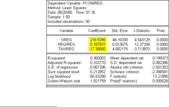
Step 2. Select Objects/New Object/Equation on the workfile menu bar, enter PCON/REG 1/REG REG/REG TAX/REG in the Equation Specification: window, and click OK. Note the coefficients highlighted in yellow.
1c=@qchisq(p,v) calculates the percentile of the χ 2 distribution . The formula finds the value c such that the prob(χ 2 with v degrees of freedom is ≤ c) = p. In this case, the prob(χ 2 with 5 degrees of freedom is ≤ 11.0704976935) =95%. In other words, 95% of the area of a χ 2 distribution, with v=5 degrees of freedom, is in the range from 0 to 11.0704976935 and 5% is in the range from 11.0704976935 to ∞ (in the tail).
2The probability value is calculated with the formula =@chisq(x,v), which returns the probability that a chi-squared statistic with v degrees of freedom exceeds x. To verify this, type the formula =@chisq(33.2256393731,5) in the EViews command window and read the value of 3.39442964858e-06 on the lower left of the EViews screen.
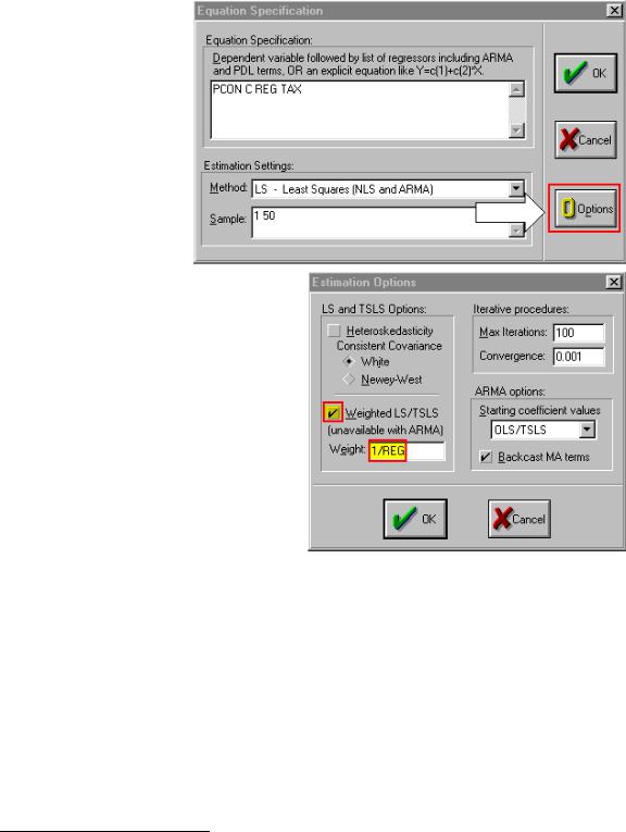
Step 3. Select Objects/New Object/Equation on the workfile menu bar and enter PCON C REG TAX in the Equation Specification: window,
and select the OOptions
button (see the arrow pointing toward the red box area in the graphic on the right).
Step 4. Check the Weighted
LS/TSLS box and enter 1/REG in the Weight: window (see the yellow highlighted and red boxed areas in the graphic on the right).
Step 5. Select OK to accept the options and select OK again to estimate the equation. Note that the weighted least squares coefficients found in Step 2 are the same as the coefficients found in Step 5 using the EViews weighted least squares option.3
3 EViews performs weighted least squares by first dividing the weight series by its mean, then multiplying all of the data for each observation by the scaled weight series. The scaling of the weight series is a normalization that has no effect on the parameter results, but makes the weighted residuals more comparable to the un-weighted residuals. The normalization does imply, however, that EViews weighted least squares is not appropriate in situations where the scale of the weight series is relevant, as in frequency weighting.
Remedies for heteroskedasticity: heteroskedasticity corrected standard errors (UE 10.4.2):
Follow these steps to estimate heteroskedasticity corrected standard errors regression:
Step 1. Open the EViews workfile named Gas10.wf1.
Step 2. Select Objects/New Object/Equation on the workfile menu bar and enter PCON C
REG TAX in the Equation Specification: window, and select the OOptions button.
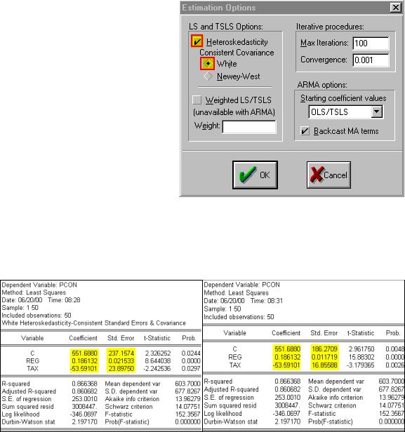
Step 3. Check the Heteroskedasticity
Consistent Covariances (White) box (see the yellow highlighted and red boxed areas in the graphic on the right).
Step 4. Select OK to accept the options and select OK again to estimate the equation.
Step 5. Compare the Estimation Output from the regression with the Heteroskedasticity Consistent Covariance on the lower left with the Estimation Output from the uncorrected OLS regression on the lower right (EQ01). Note that the coefficients are the same but the
uncorrected std. error is smaller. This means that the Heteroskedasticity Consistent Covariance correction has reduced the size of the t-statistics for the coefficients, a typical result. However, in this case both of the slope coefficients remain significant at the 5% level but the TAX variable coefficient is no longer significant at the 1% level.
Remedies for heteroskedasticity: redefining variables (UE 10.4.3):
Follow these steps to estimate UE, Equation 10.30, p. 374:
Step 1. Open the EViews workfile named Gas10.wf1.
Step 2. Select Objects/New Object/Equation on the workfile menu bar, enter PCON/POP C REG/POP TAX in the Equation Specification: window, and click OK.
Exercises:
5.Create an EViews workfile and enter the average income and average consumption data from the table printed in Exercise 5, p.378.
a.Refer to Testing for heteroskedasticity: the Park test.
b.Refer to Testing for heteroskedasticity: the Park test.
c.
d.Refer to Remedies for heteroskedasticity: heteroskedasticity corrected standard errors.
9.Open the EViews file named Books10.wf1.
c.Refer to Testing for heteroskedasticity: the Park test and Testing for heteroskedasticity: White's test.
d.Refer to Remedies for heteroskedasticity: weighted least squares.
e.Refer to Remedies for heteroskedasticity: heteroskedasticity corrected standard errors or Remedies for heteroskedasticity: redefining variables.
15.Open the EViews file named Bid10.wf1.
a.Refer to Estimate a multiple regression model using EViews and Serial Correlation (Chapter 9).
b.Refer to Serial Correlation (Chapter 9).
c.
d.Refer to Testing for heteroskedasticity: the Park test and Testing for heteroskedasticity: White's test.
e.Refer to Testing for heteroskedasticity: the Park test and Testing for heteroskedasticity: White's test.
f.

Chapter 11: A Regression User's Handbook
In this chapter:
1.A table with directions/references explaining how to view the checkpoint items displayed in UE, Table 11.1, p.391.
2.A table with directions/references explaining how to check for econometric maladies identified in UE, Table 11.2, p.393.
3.Exercise
How to observe checkpoint items displayed in UE, Table 11.1
Checkpoint |
How to observe in EViews |
X, Y |
Displaying the spreadsheet view of a group of variables |
Degrees of Freedom (df) |
To calculate the degrees of freedom for EQ01: enter the following |
|
formula in the command window, and press Enter: |
|
=EQ01.@REGOBS-EQ01.@NCOEF and view the df on the status |
|
line in the lower left of the screen |
Coefficient (β-hatk) |
EViews Estimation Output table |
t-Statistic (t) |
EViews Estimation Output table |
R-squared (R2) |
EViews Estimation Output table |
Adjusted R-squared (R-bar2) |
EViews Estimation Output table |
F-statistic (F) |
EViews Estimation Output table |
Durbin-Watson stat (DW) |
EViews Estimation Output table |
|
|
Residual (ei) |
Displaying the actual, fitted, residual, and a plot of the residuals, |
|
Graphing to detect heteroskedasticity |
S.E. of regression (SEE) |
EViews Estimation Output table |
|
|
Total sum of squares (TSS) |
To calculate the total sum of squares for a variable named Y: enter |
|
the following formula in the command window, and press Enter: |
|
series SQUAREDERROR=(Y-@MEAN(Y))^2. After that enter the |
|
following formula in the command window, and press Enter: |
|
=@SUM(SQUAREDERROR). The TSS can be viewed on the |
|
status line in the lower left of the screen. |
Sum squared resid (RSS) |
EViews Estimation Output table |
Std. Error (of coefficients) |
EViews Estimation Output table |
{SE(β-hatk)} |
|
Estimated first-order |
Using regression to estimate ρ , the first order serial correlation |
autocorrelation coefficient |
coefficient |
(ρ-hat)) |
|
Simple correlation coefficient |
Displaying the simple correlation coefficients between all pairs of |
(r12) |
variables in a group |
Variance inflation factor |
Calculating Variance Inflation Factors |
(VIF) |
|

How to check for econometric maladies identified in UE, Table 11.2
|
What's wrong |
How to check in EViews |
|
Omitted variable |
Adding or deleting variables to/from an OLS model in EViews |
|
|
|
|
Irrelevant variable |
Adding or deleting variables to/from an OLS model in EViews |
|
Incorrect functional form |
Chapter 7 Specification: Choosing A Functional Form |
|
Multicollinearity |
Chapter 8: Multicollinearity |
|
Serial correlation |
Chapter 9: Serial Correlation |
|
Heteroskedasticity |
Chapter 10: Heteroskedasticity |
|
|
|
Exercise: |
|
|
|
UE 11.7.2, pp. 406-407: |
|
Step 1. Open the EViews workfile named House11.wf1.
Step 2. Select Objects/New Object/Equation on the workfile menu bar, enter YOUR EQUATION SPECIFICATION HERE WITH THE DEPENDENT VARIABLE FIRST FOLLWOED BY C AND A LIST OF THE INDEPENDENT VARIABLE CHOSEN FOR EACH SPECIFICATION in the Equation Specification: window, and. click OK.
Step 3. Check your results for each specification, following the outline printed in UE, p. 407 (refer to the tables above for guidance on how to perform each step).

Chapter 12: Time Series Models
In this chapter:
1.Estimating ad hoc distributed lag & Koyck distributed lag models (UE 12.1.3)
2.Testing for serial correlation in Koyck distributed lag models (UE 12.2.2) using:
2.1.Durbin’s h test
2.2.The Lagrangian Multiplier (LM) test
3.Performing Granger Causality tests (UE 12.3.2)
4.Testing for nonstationarity by calculating the auto correlation function ACF (UE 12.4.1, Equation 12.24, p. 425)
5.Testing for nonstationarity with the Dickey-Fuller test (12.4.2)
6.Adjusting for nonstationarity (12.4.3)
7.Exercises
The workfile named macro14.wf1 will be used to demonstrate the procedures explained in UE, Chapter 12. The examples examine the relationship between current purchases of goods and services (CO) and the level of disposable income (YD).
Estimating an ad hoc distributed lag model (UE 12.1.3):
To estimate the ad hoc distributed lag model printed in UE, Equation 12.14, follow these steps:
Step 1. Open the EViews workfile named Macro14.wf1.
Step 2. Select Objects/New Object/Equation on the workfile menu bar, enter CO C YD(0 to -3) in the Equation Specification: window, and click OK.1
Step 3. Select Name on the equation menu bar, enter the name EQ01, and click OK. Step 4. Select Save on the workfile menu bar to save your changes.
Estimating a Koyck distributed lag model (UE 12.1.3):
To estimate the Koyck distributed lag model printed in UE, Equation 12.11, follow these steps:
Step 1. Open the EViews workfile named Macro14.wf1.
Step 2. Select Objects/New Object/Equation on the workfile menu bar, enter CO C YD CO(-1) in the Equation Specification: window, and click OK.
Step 3. Select Name on the equation menu bar, enter the name EQ02, and click OK. Step 4. Select Save on the workfile menu bar to save your changes.
1 You can include a consecutive range of lagged series by using the word "to" between the lags. YD(0 to -3) is equivalent to YD YD(-1) YD(-2) YD(-3).
Testing for serial correlation in Koyck distributed lag models using Durbin’s h test (UE 12.2.2):
Estimate the Koyck distributed lag model before attempting this section (i.e., Equation EQ02 should already be present in the workfile). To conduct a Durbin’s h test for UE, Equation 12.11, follow these steps:
Step 1. Open the EViews workfile named Macro14.wf1.
Step 2.To determine whether the value in parenthesis, in the denominator under the square root sign in UE, Equation 12.17, is positive, enter the following command in the command window:
scalar denominator=1-eq02.@regobs*(eq02.@stderrs(3)^2).
Press Enter to create a scalar object named denominator. Double click the scalar object icon named denominator in the EViews workfile and view its value in the left corner of the status bar (bottom of the EViews window). If the number is positive, continue with the next step; if not, Durbin’s h test is not valid.
Step 3.To compute Durbin’s h test statistic shown in UE, Equation 12.17, enter the following command in the command window and press Enter:
scalar dhtest=(1-(0.5*eq02.@dw))*sqr(eq02.@regobs/denominator).
Step 4. To view this scalar, double click the scalar object icon named dhtest and view its value in the left corner of the status bar (bottom of the EViews window). If the number is ≥ 1.96, reject the null hypothesis of no first order serial correlation.
Testing for serial correlation in Koyck distributed lag models using the Lagrangian Multiplier (LM) (UE 12.2.2):
Estimate the Koyck distributed lag model before attempting this section (i.e., equation EQ02 should already be present in the workfile). To conduct a Lagrangian Multiplier (LM) test for UE, Equation 12.11, follow these steps:
Step 1. Open the EViews workfile named
Macro14.wf1.
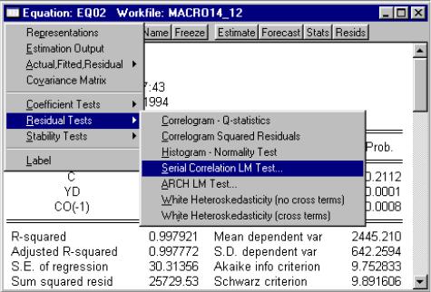
Step 2. Open the Equation named EQ02 by double clicking its icon in the workfile window.
Step 3. Select
View/Residuals
Tests/Serial Correlation LM Test… on the equation menu bar (see highlighted selections in the graphic on the right).

Step 4. Change the number in the Lags to include: to 1 in the Lag Specification: window.2 Click OK to reveal the following EViews output:
Breusch-Godfrey Serial Correlation LM Test:
F-statistic |
|
11.77690 |
Probability |
|
0.001946 |
||
Obs*R-squared |
|
9.414982 |
Probability |
|
|
0.002152 |
|
|
|
|
|
|
|
|
|
Test Equation: |
|
|
|
|
|
|
|
Dependent Variable: RESID |
|
|
|
|
|
||
Method: Least Squares |
|
|
|
|
|
|
|
Date: 07/01/00 Time: 10:25 |
|
|
|
|
|
||
Presample missing value lagged residuals set to zero. |
|
|
|
||||
Variable |
|
Coefficient |
Std. Error |
t-Statistic |
|
Prob. |
|
C |
|
-22.30297 |
26.12643 |
-0.853656 |
0.4008 |
||
YD |
|
0.113797 |
0.104157 |
1.092547 |
0.2842 |
|
|
CO(-1) |
|
-0.119235 |
0.110340 |
-1.080614 |
0.2894 |
||
RESID(-1) |
|
0.602362 |
0.175526 |
3.431748 |
0.0019 |
|
|
R-squared |
|
0.303709 |
Mean dependent var |
|
3.67E-14 |
||
Adjusted R-squared |
|
0.226343 |
S.D. dependent var |
29.28568 |
|||
S.E. of regression |
|
25.75902 |
Akaike info criterion |
9.455361 |
|||
Sum squared resid |
|
17915.24 |
Schwarz criterion |
9.640392 |
|||
Log likelihood |
|
-142.5581 |
F-statistic |
|
3.925632 |
||
Durbin-Watson stat |
|
1.630947 |
Prob(F-statistic) |
0.019027 |
|||
The null hypothesis of the LM test is that there is no serial correlation up to lag order p, where p is equal to 1 in this case. The Obs*R-squared statistic is the Breusch-Godfrey LM test statistic. This LM statistic is computed as the number of observations times the R2 from the test regression. The LM test statistic is asymptotically distributed as a χ 2 with p degrees of freedom (p is equal to 1 in this case).
Step 5. To determine whether the null hypothesis can be rejected in this case, determine the critical
χ 2(1) value from UE Table B-8. The critical χ 2 value can also be calculated in EViews by typing the following formula in the EViews command window: =@qchisq(.95,1).3 EViews returns a scalar value of 3.84. Since the calculated Breusch-Godfrey LM test statistic of 9.42 exceeds the critical χ 2(1) value, we can reject the hypothesis of no serial correlation up to lag order 1 at the 95% confidence level. The probability printed to the right of the Obs*R-squared statistic in the EViews output (i.e., 0.002152) represents the probability that you would be incorrect if you rejected the null hypothesis of no serial correlation up to lag order 1 at the 95% confidence level.
2EViews enters 2 lags by default (i.e., testing for second order serial correlation). We will enter 1 lag to estimate the LM statistic for UE, Equation 12.20, p. 421.
3c=@qchisq(p,v) calculates the percentile of the χ 2 distribution . The formula finds the value c such that the prob(χ 2 with v degrees of freedom is ≤ c) = p. In this case, the prob(χ 2 with 1 degree of freedom is ≤ 3.84) =95%. In other words, 95% of the area of a χ 2 distribution, with v=1 degrees of freedom, is in the range from 0 to 3.84 and 5% is in the range from 3.84 to ∞ (i.e., in the tail of the distribution).