

EViews Guides BITCH / EViews_tutorial
.pdfCalculating Variance Inflation Factors (UE 8.3.2):
The procedure for calculating the Variance Inflation Factors (VIF's) for explanatory variables in a regression model is explained in UE, p. 257. Use the following steps to calculate the VIF for the PF explanatory variable in UE, Equation 8.24, p. 268:
Step 1. Open the EViews workfile named Fish8.wk1.
Step 2. Select Objects/New Object/Equation on the workfile menu bar, enter PF C PB log(YD) N P in the Equation Specification: window, and click OK. Note the R2 = 0.976680.
Step 3. To save this regression, select Name on the equation window menu bar, enter EQPF in the Name to identify object: window, and click OK.
Step 4. To calculate the VIF for the variable PF, write the equation: scalar VIFPF=1/(1- EQPF.@R2) in the command window, and press Enter. The status line in the lower left of the screen will display the phrase "VIFPF successfully created." A new variable named VIFPF will appear in the workfile window.
Step 5. Double click on the VIFPF icon and the value for the Variance Inflation Factor for the variable named VIFPF = 42.88… will be displayed on the status line (lower left of the screen). The fact that VIFPF is significantly greater than 5 (i.e., the common rule of thumb value stated in UE, p. 258), would suggest that PF exhibits severe multicollinearity.
Step 6. Repeat Steps 2-5 to compute the Variance Inflation Factors for the rest of the explanatory variables in UE, Equation 8.24, p. 268.
Transforming multicollinear variables (UE 8.4.3):
Variable transformations can be achieved by creating a new variable or by simply writing the transformation in the Equation Specification: window in EViews. In many ways, the latter is preferred because the equation output labels depict the transformation.
Otherwise, it is easy to forget what transformations have been made. The table below lists the most common transformations used to rid a model of multicollinearity, along with the EViews specification (EViews specification) to make it happen.
Function Name |
Description |
|
EViews |
specification |
|||||
Linear combination |
Yt = β 0 + β 1(Xt + Zt ) |
|
|
|
|
|
Y C X+Z* |
|
|
|
|
|
|
|
|
|
|
|
|
First difference |
Yt = β 0 + β 1(Xt - Xt-1) |
|
|
|
|
|
|
Y C d(X) |
|
|
|
|
|
|
|
|
|
||
First difference of the logarithm |
Yt = β 0 + β 1(lnXt - lnXt-1) |
|
|
|
Y C dlog(X) |
|
|||
|
|
|
|
|
|
|
|
||
One-period % change (in decimal) |
Yt = β 0 + β 1[(Xt - Xt-1)/Xt ] |
|
|
|
|
Y C pch(X) |
|
||
|
|
|
|
|
|
|
|
|
|
* no spaces in the X+Z variable designation.
Exercises:
8.
a.
b. Follow the steps outlined in Detecting multicollinearity with simple correlation coefficients and Calculating Variance Inflation Factors to check for high correlations and high VIF's in the implied regression model.
13.Follow the steps outlined in Detecting multicollinearity with simple correlation coefficients and Calculating Variance Inflation Factors to check UE, Equation 8.25, p. 269 for high correlations and high VIF's.
16.
f.Run the regressions for this problem using the Mine8.wf1 data set.
a)Refer to Chapter 5 for help with this part.
b)Refer to Detecting multicollinearity with simple correlation coefficients for help with this part.
c)Refer to Transforming the multicollinear variables for help with this part.
d)Refer to Table with EViews specification for functional forms for help with this part.
Chapter 9: Serial Correlation
In this chapter:
1.Creating a residual series from a regression model
2.Plotting the error term to detect serial correlation (UE, pp. 313-315)
3.Using regression to estimate ρ , the first order serial correlation coefficient (UE, Equation 9.1, pp. 311-312)
4.Viewing the Durbin-Watson d statistic in the EViews Estimation Output window (UE 9.3)
5.Estimating generalized least squares using the AR(1) method (UE 9.4.2)
6.Estimating generalized least squares (GLS) equations using the Cochrane-Orcutt method (UE 9.4.2)
7.Exercise
Serial correlation analysis involves an examination of the error term. The demand for chicken model specified in UE, Equation 6.8, p. 166, will be used to demonstrate most of the procedures reviewed in this chapter.
Creating a residual series from a regression model:
Follow these steps to estimate the demand for chicken model (UE, Equation 6.8, p. 166), save the results in an equation named EQ01, make a residual series named E, and save changes to the workfile:
Step 1. Open the EViews workfile named Chick6.wf1.
Step 2. Select Objects/New Object/Equation on the workfile menu bar and enter Y C PC PB YD in the Equation Specification: window, and click OK.
Step 3. Select Name on the equation window menu bar, enter EQ01 in the Name to identify object: window, and click OK.
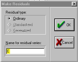
Step 4. To create a new series for the residuals (errors) for EQ01, select Procs/Make Residual Series on the equation window menu bar and the graphic on the right appears. Enter E in the Name for residual series: window, click OK, and a spreadsheet view of the residual series will be displayed in a new window.
Step 5. Select Save on the workfile menu bar to save your changes.
Plotting of the error term to detect serial correlation (UE, pp. 313-315):
Complete the section entitled Creating a residual series from a regression model before attempting this section (i.e., Equation EQ01 and series E should already be present in the workfile). Follow these steps to view a residuals graph in EViews:
Step 1. |
Open EQ01, by double clicking the |
icon in the workfile window. |
Step 2. |
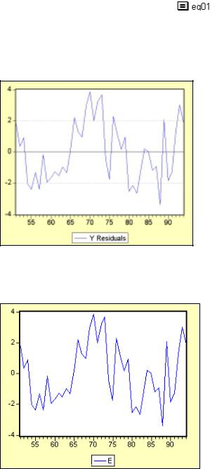
Select View/Actual, Fitted, Residual/Residual Graph on the equation window menu |
|
bar to reveal the graph on the left below. Note the residual series exhibits a pattern akin to the graphs displayed in UE, Figure 9.1, p. 313. Thus, graphical analysis indicates positive serial correlation. Steps 3 and 4 below show how to generate a time series plot of the same residual series E.
Step 3. Open the residual series named E in a new window by double clicking the series icon  in the workfile window to open the residual series from EQ01 in a new window.
Step 4. Select View/Line Graph to reveal a time series graph of the residuals shown below.
Using regression to estimate ρ , the first order serial correlation coefficient (UE, Equation 9.1, pp. 311-312):1
Complete the section entitled Creating a residual series from a regression model before attempting this section (i.e., Equation EQ01 and series E should already be present in the workfile). Follow the steps below to estimate the first order serial correlation coefficient and test for possible first order serial correlation:
Step 1. Open the EViews workfile named Chick6.wf1.
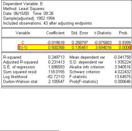
Step 2. Select Objects/New Object/Equation on the workfile menu bar, enter E C E(-1) in the Equation Specification: window, and click OK to reveal the regression output shown in the graphic below. Rho (ρ) is used to symbolize the coefficient on E(-1) and it represents the first-order autocorrelation coefficient in this regression. In this case, the value of ρ is positive and significant at the 1% level (t-statistic = 3.69 and Prob value = 0.0006). It is important to note that this is not a test of serial correlation, but the value of ρ is related to the value of the Durbin-Watson d statistic discussed in the next section.2
Step 3. Select Name on the equation menu bar, enter EQ02 in the Name to identify object: window, and click OK.
Step 4. Select Save on the workfile menu bar to save your changes.
1To test for possible second order serial correlation, regress the residuals against its value lagged one period and two periods by entering E C E(-1) E(-2) in the Equation Specification: window, and click OK. To detect seasonal serial correlation in a quarterly model, regress the residuals against its value lagged four periods enter E C E(-4) in the Equation Specification: window, and click OK. Similarly, to detect seasonal serial correlation in a monthly model, regress the residuals against its value lagged twelve periods enter E C E(-12) in the Equation Specification: window, and click OK.
2The Durbin-Watson d statistic is approximately equal to 2(1-ρ ).
Viewing the Durbin-Watson d statistic in the EViews Estimation Output window (UE 9.3):
Complete the section entitled Creating a residual series from a regression model before attempting this section (i.e., Equation EQ01 should already be present in the workfile). Follow these steps to view the Durbin-Watson d test for EQ01:
Step 1. |
Open EQ01 by double clicking the |
icon in the workfile window. |
Step 2. |
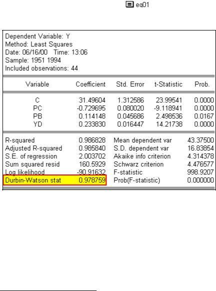
Select View/Estimation Output on the EQ01 menu bar to reveal the regression output |
|
shown below. The Durbin-Watson statistic is highlighted in yellow and boxed in red.3
Step 3. Use the Sample size printed after Included observations: (i.e., 44) and the number of explanatory variables listed in the Variable column (i.e., 3) and follow the instructions in UE, p. 612 to find the upper and lower critical d value in UE, Tables B-4, B-5 or B-6, pp. 613 - 615).
3 The Durbin-Watson statistic is a test for first-order serial correlation. More formally, the DW statistic measures the linear association between adjacent residuals from a regression model. The Durbin-Watson is
a test of the hypothesis ρ =0 in the specification:
ε t = ρε
If there is no serial correlation, the DW statistic will be around 2. The DW statistic will fall below 2 if there is positive serial correlation (in the worst case, it will be near zero). If there is negative correlation, the statistic will lie somewhere between 2 and 4. Positive serial correlation is the most commonly observed form. As a rule of thumb, with 50 or more observations and only a few independent variables, a DW statistic below about 1.5 is a strong indication of positive first order serial correlation.

Estimating generalized least squares (GLS) equations using the AR(1) method (UE 9.4.2):
Follow these steps to estimate the chicken demand model using the AR(1) method of GLS equation estimation.
Step 1. Open the EViews workfile named Chick6.wf1.
Step 2. Select Objects/New Object/Equation on the workfile menu bar, enter Y C PC PB YD AR(1) in the Equation Specification: window, and click OK to reveal the output below. EViews automatically adjusts your sample to account for the lagged data used in estimation, estimates the model, and reports the adjusted sample along with the remainder of the estimation output.
The estimated coefficients, coefficient standard errors, and t-statistics may be interpreted in the usual manner. The estimated coefficient on the AR(1) variable is the serial correlation coefficient of the unconditional residuals.4
4 Unconditional residuals are the errors that you would observe if you made a prediction of the value of using contemporaneous information, but ignoring the information contained in the lagged residual. For AR models estimated with EViews, the residual-based regression statistics—such as the, the standard error of regression, and the Durbin-Watson statistic— reported by EViews are based on the one-period-ahead forecast errors.
The most widely discussed approaches for estimating AR models are the Cochrane-Orcutt, PraisWinsten, Hatanaka, and Hildreth-Lu procedures. These are multi-step approaches designed so that estimation can be performed using standard linear regression. EViews estimates AR models using nonlinear regression techniques. This approach has the advantage of being easy to understand, generally applicable, and easily extended to nonlinear specifications and models that contain endogenous right-hand side variables.
Estimating generalized least squares (GLS) equations using the Cochrane-Orcutt method (UE 9.4.2):
The Cochrane-Orcutt method is a multi-step procedure that requires re-estimation until the value for the estimated first order serial correlation coefficient converges. Follow these steps to use the Cochrane-Orcutt method to estimate the CIA's "high" estimate of Soviet defense expenditures (i.e., this is UE, Exercise 14, Equation 9.28, p. 342).
Step 1. Open the EViews workfile named Defend9.wf1.
Step 2. Follow the steps in Creating a residual series from a regression model to estimate the OLS equation LOG(SDH) C LOG(USD) LOG(SY) LOG(SP), name it EQ01, and create a residual series for EQ01 named E.
Step 3. Estimate ρ , and name it EQ02 .
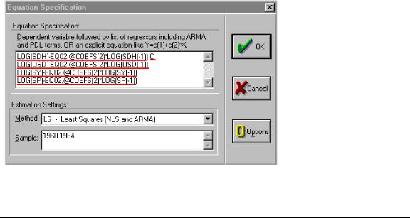
Step 4. To estimate the generalized differenced form of UE, Equation 9.28, select Objects/New Object/Equation on the workfile menu bar, enter EQ03 in the Name to identify object: window, and enter LOG(SDH)-EQ02.@COEFS(2)*LOG(SDH(-1)) C LOG(USD)-EQ02.@COEFS(2)*LOG(USD(-1)) LOG(SY)-EQ02.@COEFS(2)*LOG(SY(- 1)) LOG(SP)-EQ02.@COEFS(2)*LOG(SP(-1)) in the Equation Specification: window. The specification should appear as in the figure below.5 Click OK to view the EViews OLS output. The variable names are truncated in the EViews regression output table because they don't fit in the variable name cell. Nonetheless, the regression is correct. 6
Step 5. To calculate the new residual series, enter the following formula in the command window: series E = LOG(SDH)-(EQ03.@COEFS(1) + EQ03.@COEFS(2)*LOG(USD)
5 Statistical output for previously saved equations can be recalled by typing the equation name followed by a period and the reference to the specific output desired. In this case, the value for ρ from EQ02 (recall that ρ was coefficient # 2 on the E(-1) term) can be recalled with the command EQ02.@coefs(2). The expression EQ02.@coefs(2) can be used for ρ in the Equation Specification: window.
6 The equation can be viewed by selecting View/Representations on the equation menu bar. The equation should read: LOG(SDH)-EQ02.@COEFS(2)*LOG(SDH(-1)) = 0.1506791883 + 0.107961186*(LOG(USD)-EQ02.@COEFS(2)*LOG(USD(-1))) + 0.1368904004*(LOG(SY)- EQ02.@COEFS(2)*LOG(SY(-1))) - 0.000837025419*(LOG(SP)-EQ02.@COEFS(2)*LOG(SP(-1))). Select
View/Estimation Output on the group window menu bar to restore the estimation output view for EQ01.

+ EQ03.@COEFS(3)*LOG(SY) + EQ03.@COEFS(4)*LOG(SP)), and press Enter. The phrase "E successfully computed" should appear in the lower left of your screen.
Step 6. Re-run EQ02, EQ03 and the series E equation7 in Step 6 sequentially until the estimated ρ (i.e., the coefficient on the E(-1) term from EQ02) does not change by more that a pre-selected value such as 0.001. After 11 iterations the value for ρ converged (i.e., ρ changed from 0.957566 to 0.95758 between the 10th and 11th iteration).
Step 7. Convert the constant from the final version of EQ03 by typing the following formula in the command window: scalar BETA0=EQ03.@COEFS(1)/(1-EQ02.@COEFS(2)), and press Enter. Double click  the icon in the workfile window and read the value for the estimated constant in the lower left of the screen.
The final equation is LOG(SDH) = 3.552082480728 + 0.107961186*(LOG(USD)) + 0.1368904004*(LOG(SY)) - 0.000837025419*(LOG(SP)). Note that this is the same equation reported in UE, Exercise 14, Equation 9.28, p. 342.
Exercise:
15. Follow the steps explained in the Estimating generalized least squares (GLS) equations using the Cochrane-Orcutt method section, using SDL as the dependent variable instead of SDH.
7You can re-run an equation by opening the equation in a window, selecting Estimate on the equation menu bar, and clicking OK. You can re-run the series e equation by clicking the cursor anywhere on the equation in the command window and hitting Enter on the keyboard.
8The number 3.55208248072 was computed in Step 7 above.
Chapter 10: Heteroskedasticity
In this chapter:
1.Graphing to detect heteroskedasticity (UE 10.1)
2.Testing for heteroskedasticity: the Park test (UE 10.3.2)
3.Testing for heteroskedasticity: White's test (UE 10.3.3)
4.Remedies for heteroskedasticity: weighted least squares (UE 10.4.1)
5.Remedies for heteroskedasticity: heteroskedasticity corrected standard errors (UE 10.4.2)
6.Remedies for heteroskedasticity: redefining variables (UE 10.4.3)
7.Exercises
The petroleum consumption example specified in UE 10.5 will be used to demonstrate all aspects of heteroskedasticity covered in this guide. Data for this problem is found in EViews workfile named Gas10.wf1 and printed in Table 10.1 (UE, p. 371).
Graphing to detect heteroskedasticity (UE 10.1):
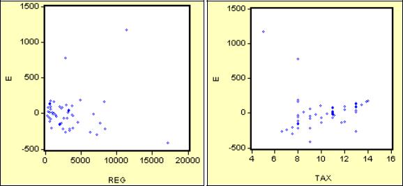
Figures 10.1, 10.2, and 10.3 in UE 10.1 demonstrate the value of a graph in detecting and identifying the source of heteroskedastic error. By graphing the residual from a regression against suspected variables, the researcher can often observe whether the variance of the error term changes systematically as a function of that variable.
Follow these steps to graph the residual from a regression against each of the independent variables in a model:
Step 1. Open the EViews workfile named Gas10.wf1.
Step 2. Select Objects/New Object/Equation on the workfile menu bar, enter PCON C REG TAX in the Equation Specification: window, and. click OK.
Step 3. Select Name on the equation menu bar, enter EQ01 in the Name to identify object: window, and click OK.
Step 4. Make a residual series named E and save the workfile.
Step 5. Make a Simple Scatter graph of E against REG to get the graph on the left below. Step 6. Make a Simple Scatter graph of E against TAX to get the graph on the right below.