

EViews Guides BITCH / EViews_tutorial
.pdfChapter 4: The Classical Model (OPTIONAL)
In this chapter:
Read this first: The procedures described in this chapter are not essential to your understanding of econometrics or to using EViews to reproduce the results published in UE. The purpose of describing the procedures in this chapter is to familiarize you with the Monte Carlo Simulation process described in (UE 4.3.2, p. 102).
Demonstrate that the estimated β s are drawn from a normal distribution (UE 4.3.2, pp. 101102):
Follow these steps to complete the process described in (UE 4.3.2):
Step 1. Open EViews and type the following commands in the command window, hitting Enter after each command:
CREATE MONTECARLO U 1 15
MATRIX(20,1) BETA
SERIES X=10+NRND
What does this do? The first command creates an undated workfile named MONTECARLO with 15 observations, the second command creates a matrix named BETA with 20 rows1 and one column to store the sample β s, and the third command creates a series named X equal to 10 plus a random number drawn from a normal distribution with zero mean and unit variance.
Step 2. Type the following commands in the command window, press Enter after each command:
SERIES Y=X+0.25*@RNORM
EQUATION EQ1.LS Y X
BETA(1)=@COEFS(1)
What this does: The first command generates a random number named y (UE, Equation 4.11, p. 101), the second command estimates the regression with y as the dependent variable and x as the independent variable (no constant), and the third command saves the β coefficient on x in the first row of the matrix named BETA. You have to repeat Step 2 for each new sample
β. However, you don’t have to re-type each line, each time. Just put the cursor on the command line and press Enter. Change the number (in parenthesis after beta in the command BETA(1)=@COEFS(1)) to the next higher number so you don’t overwrite the previous sample β . The next iteration should look like this:
SERIES Y=X+0.25*@RNORM
EQUATION EQ1.LS Y X
BETA(2)=@COEFS(1)
1 Enter the number that equals the number of sample β s you plan to estimate. The number 20 was selected for this example, but for a realistic Monte Carlo simulation, this number should be much larger.

Step 3. Type the following commands in the command window, press Enter after each command:
BETA.WRITE(T=XLS) EXCEL
CREATE BETAWF U 1 20
READ(T=XLS) EXCEL 1
RENAME SER01 BETA
BETA.HIST
SAVE
The first command writes the matrix named BETA as a series to an Excel file named EXCEL, the second command creates a new undated EViews workfile named BETAWF with 20 observations,2 the third command reads the series named excel into the EViews workfile and names it SER01, the fourth command renames SER01 to BETA, the fifth command creates a histogram of the sample β s, and the last command saves the EViews file.
2 This number should be set equal to the number of rows in the matrix named beta. See footnote 1.
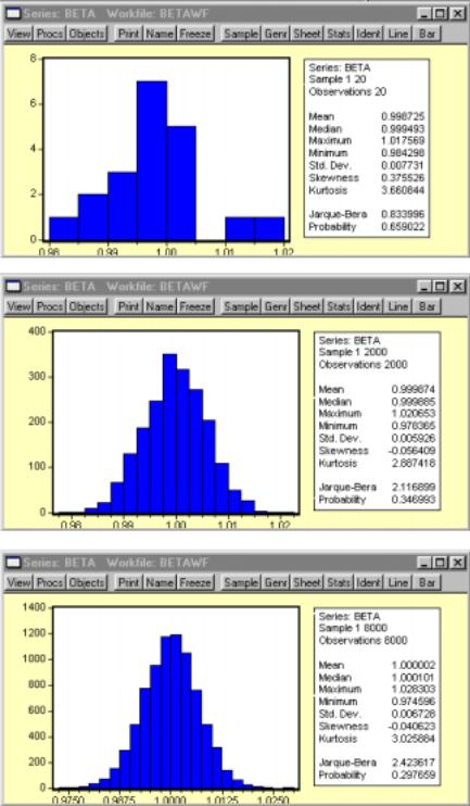
The three figures below show how the probability distribution of the estimated sample β series more closely approximates the normal distribution as the number of observations increase from 20 to 2,000 and finally to 8,000. For an explanation of the histogram and descriptive statistics represented, see Chapter 16.
The graphic on the right shows the
View/Descriptive Statistics/Histogram and Stats EViews for beta with 20 observations.
The graphic on the right shows the
View/Descriptive Statistics/Histogram and Stats EViews for beta with 2,000 observations.
The graphic on the right shows the
View/Descriptive Statistics/Histogram and Stats EViews for beta with 8,000 observations.

Chapter 5: Basic Statistics and Hypothesis Testing
In this chapter:
1.Viewing the t-value from an OLS regression (UE 5.2.1)
2.Calculating critical t-values and applying the decision rule (UE 5.2.2)
3.Calculating confidence intervals (UE 5.2.4)
4.Performing the t-test of the simple correlation coefficient (UE 5.3.3)
5.Performing the F-test of overall significance (UE 5.5)
6.Exercises
Viewing the t-value from an OLS regression (UE 5.2.1):
The Woody's Restaurants example is used to explain the use of t-values to test hypotheses concerning the coefficients on the independent variables in an OLS regression model. Follow these steps to open the Woody's Restaurant workfile in EViews and run the regression for the equation Yt = βˆ 0 + βˆ NNt + βˆ pPt + βˆ iIt + et .
Step 1. Open the EViews workfile named Woody3.wf1.
Step 2. Select Objects/New Object/Equation on the workfile menu bar, enter Y C N P I in the Equation Specification: window, and click OK. EViews generates the following output (also printed in UE, Table 3.2, p. 76):
Dependent Variable: Y
Method: Least Squares
Date: 05/23/00 Time: 05:55
Sample: 1 33
Included observations: 33 |
|
|
|
|
|
|
|
|
|
|
|
|
|
|
||||
Variable |
Coefficient |
Std. Error |
|
t-Statistic1 |
|
Prob. |
||||||||||||
|
C |
|
|
|
102192.4 |
|
|
12799.83 |
|
|
|
7.983891 |
|
|
0.0000 |
|
||
|
N |
|
|
- |
9074.674 |
|
|
2052.674 |
|
|
- |
4.420904 |
|
|
0.0001 |
|
||
|
P |
|
|
|
0.354668 |
|
|
0.072681 |
|
|
|
4.879810 |
|
|
0.0000 |
|
||
|
|
I |
|
|
|
|
1.287923 |
|
|
0.543294 |
|
|
|
2.370584 |
|
|
0.0246 |
|
R-squared |
|
|
|
0.618154 |
|
Mean |
dependent |
var |
|
|
|
125634.6 |
|
|||||
Adjusted R-squared |
0.578653 |
|
S.D. dependent var |
|
|
|
22404.09 |
|
||||||||||
S.E. of regression |
14542.78 |
Akaike info criterion |
|
|
|
22.12079 |
||||||||||||
Sum squared resid |
|
6.13E+09 |
Schwarz criterion |
|
|
|
22.30218 |
|||||||||||
Log likelihood |
-360.9930 |
|
F-statistic |
|
|
|
15.64894 |
|||||||||||
Durbin-Watson stat |
1.758193 |
|
Prob(F-statistic) |
|
|
|
0.000003 |
|||||||||||
All information needed for hypothesis testing using the t-test is found in the middle of the EViews equation output table (highlighted in yellow). The first column identifies the name of the
variable. The second column reports the estimated coefficient ( βˆ k) for each variable, and the third column reports the standard error for the estimated coefficient (SE βˆ k). The fourth column prints the calculated t-value given that the border value implied by the null hypothesis (β Ho) is zero (i.e., the t-value in this case is ( βˆ k)/(SE βˆ k)).
1 The EViews program uses the term t-Statistic rather than the term t-value, which is used in UE and this guide.

Calculating critical t-values and applying the decision rule (UE 5.2.2):
The critical t-value (tc) is the value that separates the "acceptance" region from the "rejection" region. Look up this value in UE, Statistical Table B-1, p.607. Its value depends on the degrees of freedom (printed in column one of Table B-1) and the level of Type I error specified (i.e., the number at the top of the column in Table B-1 for two-tailed tests or double the value for onetailed tests). Alternately, you can follow these steps to have EViews calculate the one-tailed and two-tailed, 5% significance level critical t-values (tc):
Step 1. Open the EViews workfile named Woody3.wf1.
Step 2. Select Objects/New Object/Equation on the workfile menu bar, enter Y C N P I in the Equation Specification: window, and click OK.
Step 3. Select Name on the equation window menu bar, enter EQ01 in the Name to identify object: window, and click OK.
Step 4. To create a vector object named result with 10 rows (to store the results of the test statistics for Woody's Restaurants regression), type the following command in the command window: vector(10) result and press Enter.2
Step 5. To compute the two-tailed critical t-value (tc) for the 5% significance level and save the value in the first row of the vector object named result, type the following equation in the command window and press Enter:3
result(1)=@qtdist(.975,(eq01.@regobs-eq01.@ncoef)).4
Step 6. To compute the one-tailed critical t-value (tc) for the 5% significance level and save the value in the second row of the vector object named result, type the following equation in the command window and press Enter:
result(2)=@qtdist(.95,(eq01.@regobs-eq01.@ncoef)).
Step 7.Double click on the Vector Object named result in the workfile window to view the two-tailed and one-tailed, 5% significance level critical t-value (tc) for the Woody's Restaurants regression. In this case, the value reported in row one of the result vector is 2.045230 and the value reported in row two is 1.69912702653.
Population was hypothesized to have a positive effect on the number of customers eating at Woody's Restaurants. This implies that the coefficient on P is expected to be positive and a one-
tailed test is appropriate. Thus, the hypothesis that the coefficient is zero ( βˆ p = 0) is rejected at
the 5% significance level because the calculated t-value (4.879810) is greater than the one-tailed critical t-value (5% level of significance), calculated in Step 6 to be 1.69912702653.
While it is important to be able to apply the decision rule by comparing the calculated t-value (reported in the EViews output) with the critical t-value just calculated, EViews makes it
2Alternately, select Objects/New Object/Matrix-Vector-Coef from the main menu or the workfile menu. Write result in the Name for Object: window, and click OK. Select Vecto in the Type window, enter 10 in the Rows window, enter 1 in the Columns window, and click OK.
3The command, @qtdist(p,v), calculates the value where the cumulative density function (CDF) of the t-distribution with (v) degrees of freedom equals (p) probability, leaving 1-p% of the t-distribution in each tail. Note that you should enter 0.975 for "p" for the two-tailed 5% significance level calculation and 0.95 for "p" for the one-tailed 5% significance level. In this case, v equals (eq01.@regobs-eq01.@ncoef), which calculates the degrees of freedom for equation eq01. The {eq01.} Part can be omitted if the calculation relates to the last regression run.
4If you omit the result(1), EViews returns a scalar value on the status line located in the lower left of your screen.

possible to test the null hypothesis that a coefficient is zero (i.e., β Ho = 0) without knowing the critical t-value. Instead, you can examine the probability (Prob.) value in the last column of the EViews OLS regression output (see the EQ01 Estimation Output table). The Prob. value shows the probability of drawing a t-value as extreme as the one actually observed when, in fact, the coefficient value is actually zero5. This probability is also known as the p-value or the marginal significance level. In terms of UE, it represents the probability of making a Type I error if the null hypothesis, that the coefficient is zero, is rejected. Given a p-value, you can tell at a glance if the null hypothesis, that the true coefficient is zero against a two-sided alternative that it differs from zero, should be rejected or accepted. For example, a p-value lower than .05 suggests rejection of the null hypothesis, for a two-tailed test at the 5% significance level. The appropriate probability is one-half that reported by EViews, for a one-sided test. This is comparable to reading the value at the top of the Critical t-Value table that is double the significance level that you are testing for a one-tailed test (i.e., using 0.10 instead of 0.05 for 5% significance level).
Applying the Prob. value, one-tailed test to the population (P) variable in the Woody's Restaurants regression, the hypothesis that the coefficient is zero ( βˆ p = 0) is rejected at the 5%
significance level if one-half of the Prob. value in the last column is less than or equal to 0.05. Note that the null hypothesis is also rejected at the 1% significance level.
Calculating confidence intervals (UE 5.2.4):
Complete steps 1-4 of the section entitled Calculating critical t-values and applying the decision rule before attempting this section (i.e., an equation object named EQ01 and a vector object named result with 10 rows should already be present in the workfile). To calculate and record the 90% confidence interval for a coefficient using EViews:
Step 1. Open the EViews workfile named Woody3.wf1.
Step 2. To calculate the lower value for the 90% confidence interval for the population coefficient, enter the following formula in the command window, and press Enter:6
result(3)= eq01.@coefs(3)-(@qtdist(.95,(eq01.@regobs-eq01.@ncoef)))*eq01.@stderrs(3).
Step 3. To calculate the upper value for the 90% confidence interval for the population coefficient, enter the following formula in the command window, and press Enter:
result(4)= eq01.@coefs(3)+(@qtdist(.95,(eq01.@regobs-eq01.@ncoef)))*eq01.@stderrs(3).
Step 4.To view the lower and upper confidence interval values, double click the vector icon named result. Note that the values 0.231175 and 0.478162 are printed in rows three and four respectively (the same values are reported in UE, p. 128).
5Under the assumption that the errors are normally distributed, or that the estimated coefficients are asymptotically normally distributed.
6eq01.@coefs(i) and eq01.@stderrs(i) are scalar values of the coefficient and standard error of the ith variable in regression eq01,where i represents the coefficient number (including the constant) listed in the EViews OLS Estimation Output. Since the population (P) variable is listed third in the Estimation Output, @coefs(3) and @stderrs(3), calculates the value for the population coefficient and its standard error respectively. As in section 5.2.2, (@qtdist(.95,(eq01.@regobs-eq01.@ncoef))) calculates the value where the cumulative density function (CDF) of the t-distribution equals 0.95 probability, leaving 5% of the t-distribution in each tail. The term (eq01.@regobs-eq01.@ncoef) calculates the degrees of freedom for EQ01, with eq01.@regobs calculating the number of observations used to estimate EQ01 and eq01.@ncoef calculating the number of coefficients estimated, including the constant.
Performing the t-test of the simple correlation coefficient (UE 5.3.3):
Complete steps 1-4 of the section entitled Calculating critical t-values and applying the decision rule before attempting this section (i.e., an equation object named EQ01 and a vector object named result with 10 rows should already be present in the workfile). To use the t-test to determine whether a particular simple correlation coefficient between Y and P is significant:
Step 1. Open the EViews workfile named Woody3.wf1.
Step 2. To calculate the simple correlation coefficient (r) and store it in the fifth row of the result vector, type the following command in the command window, and press Enter:
result(5)= @cor(y,p).
Step 3. To convert the simple correlation coefficient between Y and P into a t-value and store it in row six of the result vector, type the following command in the command window, and press
Enter: result(6) = (@cor(y,p)*((@obs(y)-2)^.5))/((1-@cor(y , p)^2)^.5).
Step 4. To calculate the critical t-value (tc) for the t-distribution with @obs(y)-2 degrees of freedom and store it in the seventh row of the result vector, type the following command in the command window, and press Enter: result(7) = @qtdist(.975,(@obs(y)-2)).
Step 5. Double click the icon for the result vector to view the results in rows 5, 6, and 7.
Performing the F-test of overall significance (UE 5.5):
Complete steps 1-4 of the section entitled Calculating critical t-values and applying the decision rule before attempting this section (i.e., an equation object named EQ01 and a vector object named result with 10 rows should already be present in the workfile). The F-statistic is reported as (15.64894) in the EQ01 estimation output table. Follow these steps to calculate the F-statistic from EQ01 and save it in row seven of a vector named result:
Step 1.Open the EViews workfile named Woody3.wf1.
Step 2. To store the F-statistic from EQ01 in row eight of the results vector, type the following command in the command window, and press Enter: result(8)=eq01.@f.
In this case, the F-statistic tests the hypothesis that all of the slope coefficients excluding the constant, in EQ01, are zero. Under the null hypothesis with normally distributed errors, this statistic has an F-distribution with k degrees of freedom in the numerator and n-k-1 degrees of freedom in the denominator, where n equals the number of observation and k equals the number of independent variables (k does not include the constant) in the model. The null hypothesis can be rejected if the calculated F-statistic exceeds the critical F-value at the chosen level of significance. The critical F-value can be determined from UE, Appendix B, Statistical Tables B- 2 or B-3, depending on the level of significance chosen. Alternately,
Step 3. To have EViews calculate the 5% critical F-value for EQ01 and store it in row nine of the results vector, type the following command in the command window, and press Enter: result(9)=@qfdist(0.95,eq01.@ncoef-1,eq01.@regobs- eq01.@ncoef).
Step 4. Double click the icon for the result vector to view the results in rows 8 and 9.
test statistic |
result row |
value |
t-critical for regression - 5% level of significance (two-tailed test) = |
R1 |
2.04523 |
t-critical for regression - 5% level of significance (one-tailed test) = |
R2 |
1.699127 |
lower confidence interval = |
R3 |
0.231175 |
upper confidence interval = |
R4 |
0.478162 |
The simple correlation coefficient (r) = |
R5 |
0.392568 |
t-calculated for correlation = |
R6 |
2.376503 |
t-critical for correlation = |
R7 |
2.039513 |
The F-statistic = |
R8 |
15.64894 |
Critical value of the F-statistic - 5% level of significance = |
R9 |
2.93403 |
|
R10 |
0 |
Since the 5% critical F-value for EQ01 (i.e., 2.934030) is significantly less than the calculated F- statistic (i.e., 15.64894), we can reject the null hypothesis that all of the slope coefficients in EQ01 are zero.
The p-value printed just below the F-statistic in the EViews regression output, denoted Prob(F- statistic), represents the marginal significance level of the F-test. If the p-value is less than the significance level you are testing, say .05, you reject the null hypothesis that all slope coefficients are equal to zero. For EQ01, the p-value is 0.000003, so we reject the null hypothesis that all of the regression coefficients are zero. Note that the F-test is a joint test so that even if all the t-values are insignificant, the F-statistic can be highly significant.
Exercises:
16.EViews can be used to complete parts 1, b, c & f of exercise 16.
a.Review the section Calculating critical t-values and applying the decision rule to learn how to use EViews to calculate the critical values for testing your hypothesis concerning the regression coefficients in this exercise.
b.Review the section Performing the F-test of overall significance to learn how to use EViews to calculate the critical value for the F-test of the overall significance of the estimated equation.
c.Review the section Calculating confidence intervals to learn how to use EViews to determine lower and upper confidence intervals for an estimated coefficient.
d.
e.
f.Review the section Using EViews to estimate a multiple regression model of beef demand in Chapter 2, if you have trouble estimating this multiple regression model using EViews.

Chapter 6: Specification: Choosing the Independent
Variables
In this chapter:
1.Adding or deleting variables to/from an OLS model in EViews (UE 6.1.2 - 6.3)
2.Lagging variables in an OLS model using EViews (UE 6.5)
3.Appendix: additional specification criteria (UE 6.8)
a.Ramsey's Regression Specification Error Test (RESET) (UE 6.8.1)
b.Ramsey's Regression Specification Error Test (RESET) (EViews)
4.Akaike's Information Criterion (AIC) and the Schwartz Criterion (SC) (EViews)
5.Exercise
Adding or deleting variables to/from an OLS model in EViews (UE 6.1.2 - 6.3):
EViews makes it easy to try alternative versions of an OLS model in order to determine whether omitting a variable is likely to result in specification bias or whether the variable is irrelevant. The four important specification criteria (UE, pp. 167-168) don't always agree. However, when the theory is not absolutely clear about the relevancy of including a specific variable in a model, the other three criteria (i.e., t-test, adjusted R2, and bias) should be considered. The only way to check these criteria is to run the regression with and without the variable and evaluate the results in terms of t-test, adjusted R2, and bias. The following steps outline a procedure to determine whether the price of beef (PB) is a relevant variable in the demand for chicken model (UE, Equation 6.8, p. 160):
Step 1. Open the EViews workfile named Chick6.wf1.
Step 2. Select Objects/New Object/Equation on the workfile menu bar, enter Y C PC PB YD in the Equation Specification: window, and click OK.
Step 3. To preserve this EViews Estimation Output view of UE, Equation 6.8, p. 160, for later comparison, select Name on the equation menu bar, enter EQ01 in the Name to identify object: window, and click OK.1
Step 4. Create a duplicate copy of EQ01 by selecting Objects/Copy object… on the EQ01 menu bar. A new UNTITLED copy of EQ01 Estimation Output appears. In this new equation window, select Estimate on the equation menu bar, delete PB from the Equation Specification: window, and click OK.
Step 5. To preserve this EViews Estimation Output of UE, Equation 6.9, p. 161, for later comparison, select Name on the equation menu bar, enter EQ02 in the Name to identify object: window, and click OK.
Step 6. Compare and evaluate the two equations based on t-statistics, adjusted R2, and bias.
1 Alternately, the EViews Estimation Output could have been preserved by selecting Freeze on the equation menu bar. The Freeze button on the objects toolbar creates a duplicate of the current view of the original object. The primary feature of freezing an object is that the tables and graphs created by freeze may be edited for presentations or reports. Frozen views do not change when the workfile sample is changed or when the data change. The purpose for freezing the regression output table is to allow us to view it later by double clicking the objects icon in the workfile window. In order to do that, the frozen object must be named.
Lagging variables in an OLS model using EViews (UE 6.5):
EViews makes it easy to lag variables in an equation.2 Equations 6.22 & 6.23 refer to a hypothetical model and they are not actually estimated in UE. However, the demand for chicken model (UE, Equation 6.8, p. 160) will be used to show how to lag variables in EViews.
Step 1. Open the EViews workfile named
Chick6.wf1.
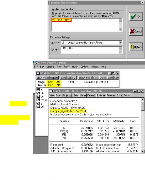
Step 2. To run the regression for Yt on PCt-1, PBt and YDt, select Objects/New Object/Equation on the workfile menu bar, enter Y C PC(-1) PB YD in the Equation Specification: window (see the graphic to the right), and click OK.
Note that EViews reports that it has adjusted the sample (see the graphic to the right). The range and sample in the workfile window show 1951 1994 but the equation output reports
Sample(adjusted):
1952 1994. You should be aware that if you include lagged variables in a regression, the degree of sample adjustment will
differ depending on whether data for the pre-sample period are available or not. For example, suppose the workfile range is 1950 1994 and the workfile sample is 1950 1994. If you specify a regression with PC lagged one period, EViews will not adjust the sample because it can use the data for 1950 in the workfile.
2 In fact, nearly any transformation of the variables using EViews functions is allowed. See
Help/Reference(Commands and Functions)/Function Reference for a list of EViews functions.