EViews Guides BITCH / EViews_tutorial

Exercises:

13.

a.

b.

c.

d.The data for this exercise are available in an EViews file named help1.wf1. However, it is a good idea to take this opportunity to make sure that you understand how to create a workfile and enter data. If you want to skip these steps, open the EViews workfile named help1.wf1 and skip steps 1 through 6 below.

Follow these steps to create a new workfile for the help-wanted advertising index (hwi) and unemployment rate (ur) data set printed in the table accompanying exercise 13.

Step 1. Select File/New/Workfile on the EViews main menu bar. Set the workfile frequency to Quarterly. Enter 1962:1 for the Start date: and 1967:4 for the End date: (see footnote 2). Click OK to open a new untitled workfile.

Step 2. To save your workfile, select Save on the workfile menu bar or File/Save or File/Save As on the main menu bar and enter help1.wf1 in the File name: window, select the destination drive in the Save in: window, and click OK.

Step 3. To create a new series for the help-wanted advertising index (hwi) variable, select Objects/New Object/Series from the main menu or the workfile menu, enter hwi in the Name for Object: window and click OK. All of the observations in the series will be assigned the missing value code 'NA'.

Step 4. To enter data into the newly created series, double click the series in the workfile window and click edit+/- on the series window menu bar. The numbers from the table can be entered to replace the NA's in the spreadsheet, pressing Enter after each entry. After the numbers have been entered, click edit+/- on the series window menu bar to save the changes and exit the edit function. The series window can be closed by clicking the button in the upper right corner of the series window.

Step 5. Repeat the process for the unemployment rate (ur) variable.

Step 6. To save changes to your workfile, click Save on the workfile menu bar.

The process of running a regression is explained, in detail, in Chapter 2, but a short description of the process is presented here. Follow these steps to run the regression between hwi and ur:

Step 1. Open the EViews workfile named Help1.wf1.

Step 2. Select Objects/New Object/Equation and click OK (or Quick/Estimate Equation from the main menu).

Step 3. Enter the dependent variable (hwi), the constant (c) and the independent variable (ur) in the Equation Specification: window that appears, using spaces between each term. It is important to enter the dependent variable first (hwi in this case).

Step 4. Select the estimation method {LS - Least Squares (NLS and ARMA)}. EViews uses this as the default setting because it is selected most of the time.

Step 5. The workfile sample range is automatically entered but it can be changed if another sample range is desired.

Step 6. Click OK when finished to reveal the regression output generated by EViews.

Chapter 2: Ordinary Least Squares

In this chapter:

1.Running a simple regression for weight/height example (UE 2.1.4)

2.Contents of the EViews equation window

3.Creating a workfile for the demand for beef example (UE, Table 2.2, p. 45)

4.Importing data from a spreadsheet file named Beef 2.xls

5.Using EViews to estimate a multiple regression model of beef demand (UE 2.2.3)

6.Exercises

Ordinary Least Squares (OLS) regression is the core of econometric analysis. While it is important to calculate estimated regression coefficients without the aid of a regression program one time in order to better understand how OLS works (see UE, Table 2.1, p.41), easy access to regression programs makes it unnecessary for everyday analysis.1 In this chapter, we will estimate simple and multivariate regression models in order to pinpoint where the regression statistics discussed throughout the text are found in the EViews program output. Begin by opening the EViews program and opening the workfile named htwt1.wf1 (this is the file of student height and weight that was created and saved in Chapter 1).

Running a simple regression for weight/height example (UE 2.1.4):

Regression estimation in EViews is performed using the equation object. To create an equation object in EViews, follow these steps:

Step 1. Open the EViews workfile named htwt1.wf1 by selecting File/Open/Workfile on the main menu bar and click on the

file name.

Step 2. Select Objects/New Object/Equation from the workfile menu.2

Step 3. Enter the name of the equation (e.g., EQ01) in the Name for Object: window and click OK.

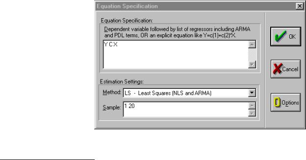
Step 4. Enter the dependent variable weight (Y), the constant (C) and the independent variable height (X) in the Equation Specification: window (see

figure on right). It is important to enter the dependent variable first (Y in this case).

1Using Econometrics, A Practical Guide (fourth edition), by A. H. Studenmund will be referred to as (UE) when referenced in this guide.

2Alternately, select Quick/Estimate Equation from the main menu. If this method is used, the equation must be named to save it. Click Name on the equation menu bar and enter the desired name and click OK.

Step 5. Select the estimation Method {LS - Least Squares (NLS and ARMA)}. This is the default that will be used most of the time.

Step 6. The workfile sample range is automatically entered but it can be changed if another sample range is desired. Click OK to view the EViews Least Squares regression output table.

Step 7. To save changes to your workfile, click Save on the workfile menu bar.

Contents of the EViews equation window:

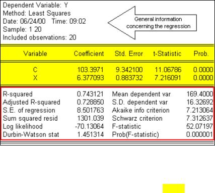
Most of the important statistical information relating to a regression is reported in the EViews equation window (see the figure below). General information concerning the regression is printed in the top few lines, the coefficient statistics are reported in table format (middle five columns), and summary statistics are printed in table format (bottom four columns) of the equation window.

General Information Printed in the Top Portion of the Equation Output: The first five or six lines identify (see arrow

in figure on right): Line 1. Name of the dependent variable.

Line 2. Regression method used.

Line 3. Date & time the regression was executed. Line 4. Sample range used in the regression.

Line 5. Number of observations included in your regression.

Line 6. Number of excluded observations.

Line 6 is not reported in this

case because no observations are excluded (i.e., no variable, included in the regression, has missing observations or is lagged with data not available for the pre-sample period).

Coefficient Results: Key information regarding the estimated regression coefficients is reported in a table displayed in the middle of the regression output (see area highlighted in yellow). The first column identifies each variable (C for the constant and X for height) and the second column

reports the estimated coefficient values (i.e., βˆ o & βˆ 1). Note that the estimated coefficients are

the same as those printed in (UE, Equation 1.21, pp. 20 & 21). The data printed in columns (3) -

(6) are the standard error of the coefficient, the t-statistic and the probability respectively. We will not discuss these now, but they will be very important when Hypothesis Testing is discussed in Chapter 5.

Summary Statistics: Key summary statistics are reported in four columns below the equation output (see area outlined in red). Each will be defined and the page reference to where it is discussed in UE is identified in parenthesis.

1.R2 : coefficient of determination is the fraction of the variance of the dependent variable

explained by the independent variables (p. 50);

2.R 2 : adjusted R2 (p. 51);

3.Standard Error of the Regression (S.E. of regression): called Standard Error of Estimate

(SEE) in UE (p. 105t & 392t);

4.Sum of squared resid: OLS selects the value of the coefficients to minimize this (pp. 37− 38);

5.Log likelihood: useful in hypothesis testing;

6.Durbin-Watson stat: test statistic for serial correlation in the residuals (p.324);

7.Mean dependent var: measure of central tendency for the dependent variable (pp. 522-526);

8.S.D. dependent var: measure of dispersion (Standard Deviation) for the dependent variable (pp. 526-529);

9.Akaike info criterion: used in model selection (pp. 195-197);

10.Schwarz criterion: used in model selection (pp. 195-197);

11.F-statistic: tests the hypothesis that all of the slope coefficients (excluding the constant, or intercept) in a regression are zero (pp. 142− 145);

12.Prob(F-statistic): (pp. 144− 145).

Multivariate Regression (2.2.3):

Multivariate regression is executed the same as simple regression in EViews and the output is identical. In this section we create a workfile, import data from a spreadsheet and estimate a multivariate regression model using the Beef example (UE, p. 45).

Creating a workfile for the demand for beef example (UE, Table 2.2, p. 45):

Note that Table 2.2 reports annual data for the price and quantity of beef and disposable personal income for the period 1960 through 1987. To create an EViews workfile:

Step 1. Select File/New/Workfile on the main menu.

Step 2. Set the Workfile frequency: to Annual.

Step 3. Enter the Start date: (1960) and End date: (1987).

Step 4. Click OK.

Importing data from a spreadsheet file named Beef2.xls:

Once the workfile has been created, it is a simple matter to import data from another file. However, you must first know the location of the data in the spreadsheet file.

To view the location of the data in the spreadsheet file:

Step 1. Open the Excel program and then open the Excel spreadsheet file named Beef2.xls, located on the Addison Wesley Longman web site. You can get there by clicking this

http://occ.awlonline.com/bookbind/pubbooks/studenmund_awl/ URL. Click on the Student Resources/Data

Sets/Data Sets-Excel. You must be connected to the internet for this link to work.

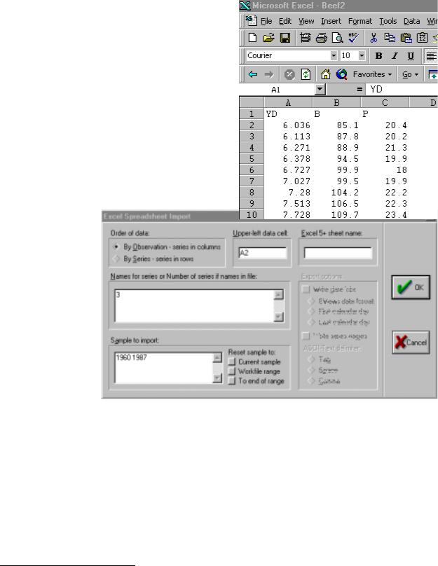
Step 2. Note that the first data series starts in cell A2 and that the data are in three contiguous columns (see the figure below).

Follow these steps to import the data from the

Beef2.xls Excel file into your new EViews file:

Step 1. Close the spreadsheet file (two programs cannot access the same file at the same time).

Step 2. Click Procs/Import/Read Text-Lotus-Excel on the workfile menu bar3.

Step 3. Select the drive and folder location in the Look in: window.

Step 4. Select Excel.xls in the Files of type: window. Step 5. Double click on the file named Beef2.xls. Step 6. Fill in A2 for the upper left data cell and 3 for

the number of series (note that when you enter the number of series, EViews will enter the names of the series that are printed in the row above each data series).

Step 7. The sample range is set to the workfile sample by default. The screen should look like the figure on the right.

Step 8. Click OK to complete the import process. If you get an error message that reads 'Unable to open file …' it means that you probably have not closed the file in

Excel. If the error message does not display, the data was successfully imported.

Using EViews to estimate a multiple regression model of beef demand (UE 2.2.3):

To Regress Beef Demand (B) on the Constant (C), the Price of Beef (P) and Per Capita Disposable Income (Yd):

Step 1. Open the EViews workfile named Beef2.wf1.

Step 2. Select Objects/New Object/Equation on the workfile menu bar and enter B C P Yd in the Equation Specification: window. Do not change the default settings for Method and Sample.

3 If you know the location and name for the spreadsheet file, you can skip steps 3− 5. Instead, fill in the File name box and click OK.

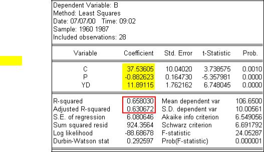
Step 3. Click OK to get the regression results shown in the table on the right. Check the coefficients in column 2 of the EViews, Least Squares output table (highlighted in yellow) with the results reported in UE, Equation 2.10, p. 44.

Describing the Overall Fit

of the Estimated Model

(UE 2.4):

R2, the coefficient of determination and R2, the adjusted R2, are located right

under the coefficients column of the table printed in the middle of the EViews regression output (outlined in red). In this case, R2 = 0.66 and R2 = 0.63.

Exercises:

4.Follow the steps described in Chapter 1 of the EViews guide to create an EViews workfile and enter the data into an EViews workfile. Follow the steps described in Running a simple regression for weight/height example of the EViews guide to regress per capita income as a function of percent of labor in agriculture on farms.

Chapter 3: Learning To Use Regression Analysis

In this chapter:

1.Displaying the spreadsheet view of a group of variables (UE, Table 3.1)

2.Displaying the descriptive statistics for a group of variables (UE, Table 3.1)

3.Displaying the simple correlation coefficients between all pairs of variables in a group (UE, Table 3.1)

4.Running a simple regression for Woody's Restaurants example (UE, Table 3.2)

5.Documenting the results

6.Displaying the actual, fitted, residual, and a plot of the residuals (UE, Table 3.2)

The Woody's Restaurants data will be used to show how EViews can be used to do the items listed above. The steps required to display the 'spreadsheet view', descriptive statistics, and simple correlation coefficients between all pairs of variables in a group are as follows:

Displaying the spreadsheet view of a group of variables (UE, Table 3.1):

Step 1. Open the EViews workfile named Woody3.wf1 by clicking File/Open/Workfile on the main menu and double click on the file named Woody3.wf1.

Step 2.To Create an EViews group for the Woody's Restaurants example, hold down the Ctrl button, click on Y, N, P & I, select Show from the workfile toolbar, and click OK.

Step 3. When you click OK, EViews displays the spreadsheet view of the data for the variables included in the group (i.e., Y, N, P & I in this case). EViews allows you to change the view with the click of a button. If you are in another view, you can display the spreadsheet view by clicking View/Spreadsheet on the group window menu bar.

Step 4. Click Name on the group menu bar and enter GROUP01 in the Name to identify object: window.1

Displaying the descriptive statistics for a group of variables (UE, Table 3.1):

Step 1. Open the group object created in Display the spreadsheet view of a group of variables by double clicking the icon in the workfile window.

Step 2. Click View/Descriptive Stats/Individual Samples on the group window menu bar to view descriptive statistics for GROUP 01.2

1 You must name a group object if you want to keep its results. Unnamed objects are labeled “UNTITLED” and the results are lost when the object window or the workfile is closed. To name a group, click Name on the group menu bar and enter the name in the Name to identify object: window. Once named, a 'group object' is saved with the

workfile and can be viewed by double clicking its icon (i.e., ) in the workfile window. 2 The group view drop-down menu is divided into four blocks:

·The views in the first block provide various ways of looking at the actual data in the group.

·The views in the second block display various basics statistics.

·The views in the third block are for specialized statistics for time series data.

·The fourth block contains the label view, which provides information regarding the group object.

The descriptive statistics printed in the table below are defined in footnote 3 at the bottom of this page.3 See Chapter 16 to gain a better understanding of these statistics.

Step 3. Select View/Spreadsheet on the group window menu bar to restore the spreadsheet view for

GROUP 01.

Displaying the simple correlation coefficients between all pairs of variables in a group (UE, Table 3.1):

Step 1. Open the group object created in Display the spreadsheet view of a group of variables by double clicking the icon in the workfile window.

Step 2.Click View/Correlations on the group window menu bar to display the simple correlation coefficients between all pairs of variables included in the group object (see the table below).4

3 All of the statistics are calculated using observations in the current sample.

Mean is the average value of the series, obtained by adding up the series and dividing by the number of observations. Median is the middle value (or average of the two middle values) of the series when the values are ordered from the smallest to the largest. The median is a robust measure of the center of the distribution that is less sensitive to outliers than the mean. Max and Min are the maximum and minimum values of the series in the current sample. Std. Dev. (standard deviation) is a measure of dispersion or spread in the series. Skewness is a measure of asymmetry of the distribution of the series around its mean. Kurtosis measures the peakedness or flatness of the distribution of the series. Jarque-Bera is a test statistic for testing whether the series is normally distributed. The test statistic measures the difference of the skewness and kurtosis of the series with those from the normal distribution. Under the null hypothesis of a normal distribution, the Jarque-Bera statistic is distributed as with 2 degrees of freedom. The reported Probability is the probability that a Jarque-Bera statistic exceeds (in absolute value) the observed value under the null—a small probability value leads to the rejection of the null hypothesis of a normal distribution.

4 View/Correlations displays the correlation matrix of the series in the selected group. Observations for which any one of the series has missing data are excluded from the calculation.

Running a simple regression for Woody's Restaurants example (UE 3.2):

To regress the number of customers served (Y) on the Constant (C), the number of direct market competitors within a two-mile radius of the Woody's location (N), the number of people living within a three-mile radius of the Woody's location (P), and the average household income of people living within a three-mile radius of the Woody's location (I):

Step 1. Open the EViews workfile named Woody3.wf1.

Step 2. To estimate UE, Equation 3.6, p. 74, select Objects/New Object/Equation on the workfile menu bar.5 You can name the equation object now by deleting Untitled in the Name for Object: window and typing a name for the equation you are about to estimate, or you can skip this step and name the equation later (if you find that it is worth saving). Click OK to reveal the Equation Specification: window.

Step 3. Enter Y C N P I in the Equation Specification: window. Step 4. Do not change the default settings for Method: and Sample:.

Step 5. Click OK to get the computer output printed in the top box of UE, Table 3.2, p. 76. Step 6. To name the equation for later use, select Name on the equation window menu bar, enter

EQ01 in the Name to identify object: window, and click OK.6

Documenting the results:

All of the data necessary to write the results printed in (UE, Equation 3.7, p. 77) are printed in the EViews regression output. EViews provides a variety of views for regression results. For example, if you are documenting the results in a word processing file, you can facilitate the process by clicking View/Representations on the equation window menu bar to get the following:

Estimation Command:

=====================

LS Y C N P I

Estimation Equation:

=====================

Y = C(1) + C(2)*N + C(3)*P + C(4)*I

Substituted Coefficients:

=====================

Y = 102192.4277 - 9074.674399*N + 0.3546683674*P + 1.287923391*I

You can copy the last line and paste it into your word processing file to get the first line of UE, Equation 3.7.

5Alternately, select Quick/Estimate Equation from the main menu. If this method is used, you must name the equation to save it. Click Name on the equation menu bar and enter the desired name in the Name for object: window and click OK.

6Restrictions on naming an object include, the name cannot exceed 16 characters and it cannot be a reserved name. The following names are reserved and should not be used for series: ABS, ACOS, AR, ASIN, C, CON, CNORM, COEF, COS, D, DLOG, DNORM, ELSE, ENDIF, EXP, LOG, LOGIT, LPT1, LPT2, MA, NA, NRND, PDL, RESID, RND, SAR, SIN, SMA, SQR, and THEN.

Select View/Estimation Output on the group window menu bar to restore the estimation output view for EQ01.

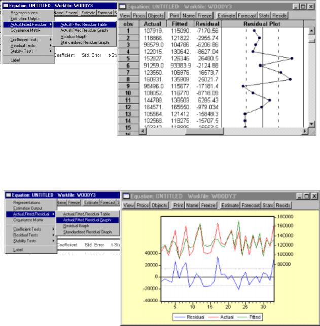
Displaying the actual, fitted, residual, and a plot of the residuals for a regression (see UE, Table 3.2, p. 76):

Step 1. Open the EViews workfile named Woody3.wf1 and open the equation named EQ01 by double clicking the equation icon in the workfile window.

Step 2a. Click View/Actual,Fitted,Residual/Actual,Fitted,Residual Table on the equation window menu bar (see figure below left). Click OK to reveal the figure below right.

Step 2b. Alternately, to display a graph of the actual, fitted, and residuals for a regression, click

View/Actual,Fitted,Residual/Actual,Fitted,Residual Graph (see figure below left). Click OK to reveal the figure below right. Other views available in the equation window will be explained in future chapters of this guide.