Chapter 17. Odds and Ends
An odds and ends chapter is a good spot for topics and tips that don’t quite fit anywhere else. You’ve heard of Frequently Asked Questions. Think of this chapter as Possibly Helpful Auxiliary Topics.
Daughter hint: Oh daddy, that’s so 90’s.
How Much Data Can EViews Handle?
EViews holds workfiles in internal memory, i.e., in RAM, as opposed to on disk. Eight bytes are used for each number, so storing a million data points (1,000 series with 1,000 observations each, for example) requires 8 megabytes.
Data capacity isn’t an issue unless you have truly massive data needs, perhaps processing public use samples from the U.S. Census or records from credit card transactions. Current versions of EViews for 32-bit machines do have an out-of-the box limit of 4 million observations per series. If you are working on a 64-bit machine, you will be limited to 120 million observations per series.
Hint: Student versions of EViews place limits on the amount of data that may be saved and omit some of EViews’ more advanced features.
How Long Does It Take To Compute An Estimate?
Probably not long enough for you to care about.
On the author’s somewhat antiquated PC, computing a linear regression with ten right-hand side variables and 100,000 observations takes roughly one eye-blink.
Nonlinear estimation can take longer. First, a single nonlinear estimation step, i.e., one iteration, can be the equivalent of computing hundreds of regressions. Second, there’s no limit on how many iterations may be required for a nonlinear search. EViews’ nonlinear algorithms are both fast and accurate, but hard problems can take a while.
Freeze!
EViews’ objects change as you edit data, change samples, reset options, etc. When you have table output that you want to make sure won’t change, click the  button to open a new window, disconnected from the object you’ve been working on—and therefore frozen.
You’ve taken a snapshot. Nothing prevents you from editing the snapshot—that’s the stan-
394—Chapter 17. Odds and Ends
dard approach for customizing a table for example—but the frozen object won’t change unless you change it.
Hint: Any untitled EViews object will disappear when you close its window. If you want to keep something you’ve frozen, use the  button.
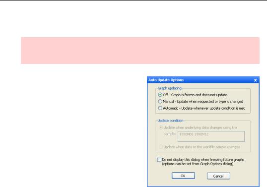
Frozen graphs offer more sophisticated behavior than frozen tables. When you have graphical output and click on the  button, EViews opens a dialog prompting you to choose Auto Update Options. Selecting Off means that the frozen graph acts exactly like a frozen table; it is a snapshot of the current graph that is disconnected from the original object. If you choose Manual or Automatic EViews will create a frozen (“chilled”) graph snapshot of the current graphical output that can update itself when the data in the original object changes.
Every frozen object is kept either as a table,
shown in the workfile window with the  icon, or a graph, shown with the
  icon. No matter how an object began life, once frozen you can adjust its appearance by using customization tools for tables or graphs.
A Comment On Tables—395
A Comment On Tables
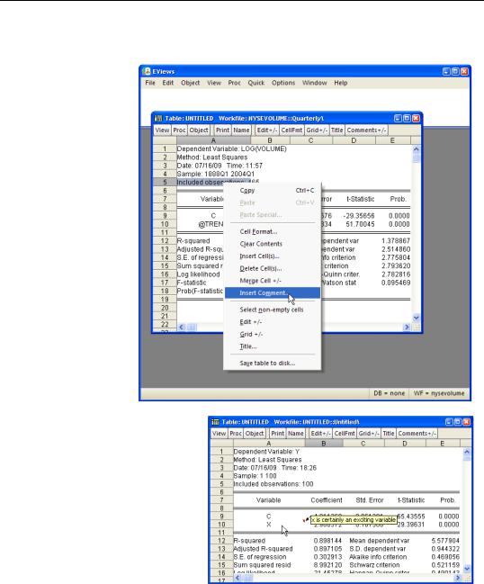
Every object has a label view providing a place to enter remarks about the object. Tables take this a step further. You can add a comment to any cell in a table. Select a cell and choose
Proc/Insert/Edit Comment… or right-click on a cell to bring up the context menu.
Cells with com-
ments are marked with little red triangles in the upper righthand corner. When the mouse passes over the cell, the comment is displayed in a note box.
396—Chapter 17. Odds and Ends
Saving Tables and Almost Tables
It’s nice to look at output on the screen, but eventually you’ll probably want to transfer some of your results into a word processor or other program. One fine method is copy-and-paste. You can also save any table as a disk file through Proc/Save table to disk… or the Save table to disk… context menu item when you
right-click in the table. Either way, you get a nice list of choices for the table format on disk.
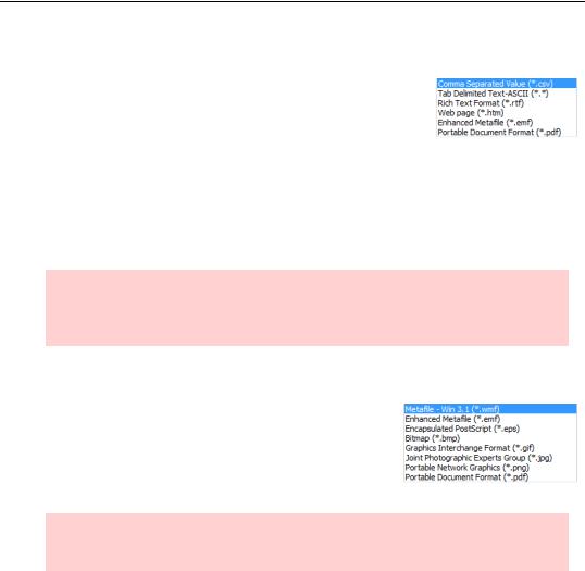
If you’re planning on reading the table into a spreadsheet or database program, choose
Comma Separated Value or Tab Delimited Text-ASCII. If the table’s eventual destination is a word processor, you can use Rich Text Format to preserve the formatting that EViews has built into the table.
Hint: If you’re looking at a view of an object that would become a table if you froze it—regression output or a spreadsheet view of a series are examples—Save table to disk… shows up on the right-click menu even though it isn’t available from Proc.
Saving Graphs and Almost Graphs
Saving graphs works much like saving tables. In addition to using copy-and-paste to transfer your graph into another program, you can save any graph as a disk file through
Proc/Save graph to disk… or the Save graph to disk… context menu item when you right-click in the graph. Simply select one of the available graph disk formats.
Hint: If you’re looking at a view of an object that would become a graph if you froze it—Save graph to disk… shows up on the right-click menu.