Loopy—385
Loopy
Program loops are a powerful method of telling EViews to repeatedly execute commands without you having to repeatedly type the commands. Loops can use either control variables or string variables.
A loop begins with a for command, with the rest of the line defining the successive values to be taken during the loop. A loop ends with a next command. The lines between for and next are executed for each specified loop value. Most commonly, loops with control variables are used to execute a set of commands for a sequence of numbers, 0, 1, 2,…. In contrast, loops with string variables commonly run the commands for a series of names that you supply.
Number loops
The general form of the for command with a control variable is:
for !control_variable=!first_value to !last_value step !stepvalue
'some commands go here
next
If the step value is omitted, EViews steps the control variable by 1.
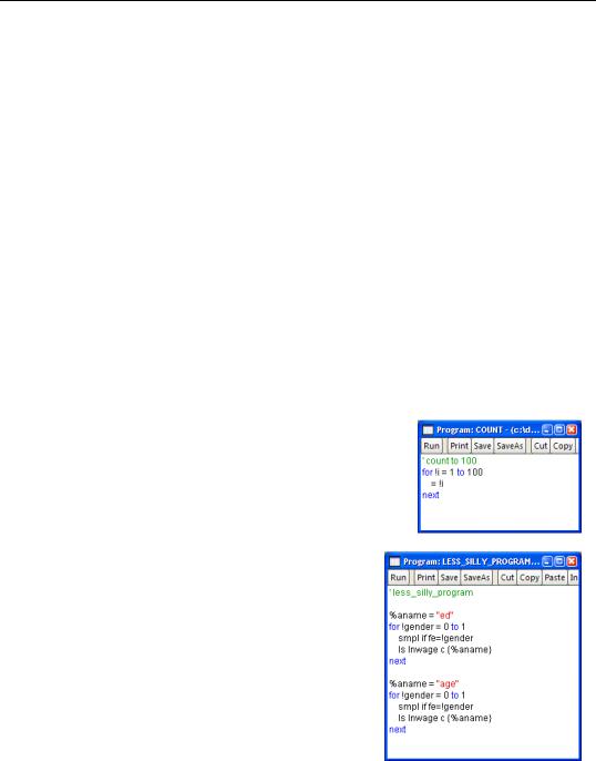
The program “count.prg” counts to 100, displaying the count on the status line. Most econometricians can count to 100 on their own, so this program is rarely seen in the wild. We captured this unusual specimen because it provides a particularly pristine example of a numerical loop.
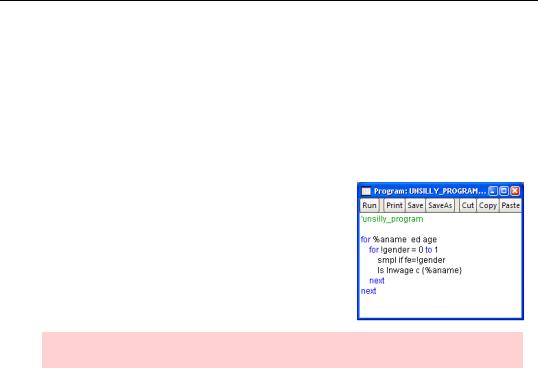
For something a bit more likely to be of practical use, we’ve simplified “silly_program.prg” by putting the values 0 and 1 in a loop instead of writing out each statement twice. In “less_silly_program.prg”, !GENDER is the control variable, !FIRST_VALUE is 0 and !LAST_VALUE is 1.
String Loops
A for command with a string variable has a string variable followed by a list of strings (no equal sign).
386—Chapter 16. Get With the Program
Each string is placed in turn in the string variable and the lines between for and next are executed.
for %string string1 string2 string3
'some commands go here
next
The commands between for and next are executed first with the string “string1” replacing “%string”, then with “string2”, etc.
To further simplify “less_silly_program.prg” so that we don’t have to write our code separately for ED and for AGE, we can add a for command with a string variable.
Hint: Loops are much easier to read if you indent.
Other Program Controls
In addition to the command form used throughout EViews Illustrated, commands can also be written in “object form.” In a program, use of the object form is often the easiest way to set options that would normally be set by making choices in dialog boxes.
Sometimes you don’t want the output from each command in a program. For example, in a Monte Carlo study you might run 10,000 regressions, saving one coefficient from each regression for later analysis, but not otherwise using the regression output. (A Monte Carlo study is used to explore statistical distributions through simulation techniques.) Creating 10,000 equation objects is inefficient, and can be avoided by using the object form. For example, the program:
for !i = 1 to 10000
ls y c x
next
runs the same regression 10,000 times, creating 10,000 objects and opening 10,000 windows. (Actually, you aren’t allowed to open 10,000 windows, so the program won’t run.) The program:
equation eq
for !i = 1 to 10000
A Rolling Example—387
eq.ls y c x
next
uses the object form and creates a single object with a single, re-used window.
Hint: Prefacing a line in a program with the word do also suppresses windows being opened. do doesn’t affect object creation.
EViews offers other programming controls such as if-else-endif, while loops, and subroutines. We refer you to the Command and Programming Reference.
A Rolling Example
Here’s a very practical problem that’s easily handled with a short program. The workfile “currency rolling.wf1” has monthly data on currency growth in the variable G. The commands:
smpl @all
ls g c g(-1)
fit gfoverall
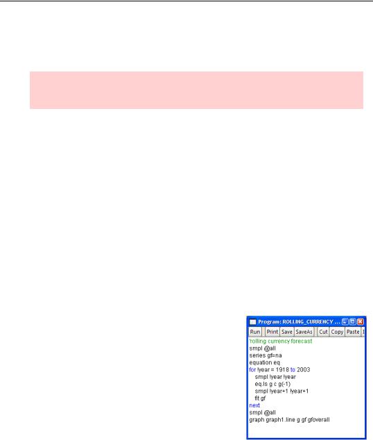
estimate a regression and create a forecast. Of course, this example uses current data to estimate an equation, which is then used to forecast for the previous century. We might instead perform a rolling regression, in which we estimate the regression over the previous year, use that regression for a one year forecast, and then do the same for the following year.
The program “rolling_currency.prg”, shown to the right, does what we want. Note the use of a for loop to control the sample—a common idiom in EViews. Note also that we “re-used” the same equation object for each regression to avoid opening multiple windows.
388—Chapter 16. Get With the Program
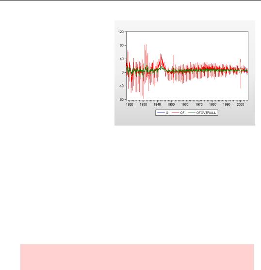
For this particular set of data, the rolling forecasts are much closer to the actual data than was the overall forecast.
Quick Review
An EViews program is essentially a list of commands available to execute as needed. You can make the commands apply to different objects by providing arguments when you run the program. You can also automate repetitive commands by using numerical and string “for…next” loops. An EViews program is an excellent way to document your operations, and compared to manually typing every command can save a heck of a lot of time!
Nearly all operations can be written as commands suitable for inclusion in a program. Simple loops are quite easy to use. A limited set of matrix operations are available for more complex calculations. However, it’s probably best to think of the program facility as providing a very sophisticated command and batch scripting language rather than a full-blown programming environment.
And if you come across a need for something not built in, see the—no, not the User’s Guide this time—see the 900+page Command and Programming Reference.
Hint: If you want to learn more about writing EViews programs, start with Chapter 17, “EViews Programming” in the User’s Guide.
Appendix: Sample Programs
Rolling forecasts
The dynamic forecast procedure for an equation produces multi-period forecasts with the same set of estimated parameters. Suppose instead that you want to produce multi-period forecasts by reestimating the parameters as new data become available. To be more specific, suppose you want to produce forecasts up to 4 periods ahead from each subsample where each subsample is moved 4 periods at a time.
Appendix: Sample Programs—389
The following program uses a for loop to step through the forecast periods. Notice how smpl is used first to control the estimation period, and is then reset to the forecast period. Temporary variables are used to get around the problem of the forecast procedure overwriting forecasts from earlier windows.
'set window size !window = 20
'get size of workfile !length = @obsrange
'declare equation for estimation equation eq1
'declare series for final results
series |
yhat ' |
point estimates |
series |
yhat_se' |
forecast std.err. |
'set step size !step = 4
'move sample !step obs at a time
for !i = 1 to !length-!window+1-!step step !step
'set sample to estimation period smpl @first+!i-1 @first+!i+!window-2
'estimate equation
eq1.ls y c y(-1) y(-2)
' reset sample to forecast period
smpl @first+!i+!window-1 @first+!i+!window-2+!step
'make forecasts in temporary series first eq1.forecast(f=na) tmp_yhat tmp_se
'copy data in current forecast sample yhat = tmp_yhat
yhat_se = tmp_se
next
Monte Carlo
Earlier in the chapter, we briefly touched on the idea of a Monte Carlo study. Here’s a more in depth example.
A typical Monte Carlo simulation exercise consists of the following steps:
1.Specify the “true” model (data generating process) underlying the data.
2.Simulate a draw from the data and estimate the model using the simulated data.
3.Repeat step 2 many times, each time storing the results of interest.
390—Chapter 16. Get With the Program
4.The end result is a series of estimation results, one for each repetition of step 2. We can then characterize the empirical distribution of these results by tabulating the sample moments or by plotting the histogram or kernel density estimate.
The following program sets up space to hold both the simulated data and the estimation results from the simulated data. Then it runs many regressions and plots a kernel density for the estimated coefficients.
'store monte carlo results in a series
'checked 4/1/2004
'set workfile range to number of monte carlo replications wfcreate mcarlo u 1 100
'create data series for x
'NOTE: x is fixed in repeated samples
'only first 10 observations are used (remaining 90 obs missing) series x
x.fill 80, 100, 120, 140, 160, 180, 200, 220, 240, 260
'set true parameter values
!beta1 = 2.5 !beta2 = 0.5
'set seed for random number generator rndseed 123456
'assign number of replications to a control variable !reps = 100
'begin loop
for !i = 1 to !reps
'set sample to estimation sample smpl 1 10
'simulate y data (only for 10 obs) series y = !beta1 + !beta2*x + 3*nrnd
'regress y on a constant and x equation eq1.ls y c x
'set sample to one observation
smpl !i !i
' and store each coefficient estimate in a series series b1 = eq1.@coefs(1)
series b2 = eq1.@coefs(2)
Appendix: Sample Programs—391
next
'end of loop
'set sample to full sample smpl 1 100
'show kernel density estimate for each coef freeze(gra1) b1.kdensity
'draw vertical dashline at true parameter value gra1.draw(dashline, bottom, rgb(156,156,156)) !beta1 show gra1
freeze(gra2) b2.kdensity
' draw vertical dashline at true parameter value gra2.draw(dashline, bottom, rgb(156,156,156)) !beta2 show gra2
Descriptive Statistics By Year
Suppose that you wish to compute descriptive statistics (mean, median, etc.) for each year of your monthly data in the series IP, URATE, M1, and TB10. One approach would be to link the data into an annual page, see Chapter 9, “Page After Page After Page,” and then compute the descriptive statistics in the newly created page.
Here’s another approach, which uses the statsby view of a series to compute the relevant statistics in two steps: first create a year identifier series, and second compute the statistics for each value of the identifier.
'change path to program path %path = @runpath
cd %path
'get workfile
%evworkfile = "..\data\basics" load %evworkfile
'set sample smpl 1990:1 @last
'create a series containing the year identifier series year = @year
'compute statistics for each year and
'freeze the output from each of the tables
for %var ip urate m1 tb10 %name = "tab" + %var
392—Chapter 16. Get With the Program
freeze({%name}) {%var}.statby(min,max,mean,med) year
show {%name}
next
More Samples
These sample programs were all taken from online help, found under Help/Quick Help Reference/Sample Programs & Data. Over 50 programs, together with descriptions and related data, are provided. Reading the programs is an excellent way to pick up advanced techniques.