


Chapter 2. EViews—Meet Data
When you embark on an econometric journey, your first step will be to bring your data into EViews. In this chapter we talk about a variety of methods for getting this journey started on the right foot.
Unlike the blank piece of paper that appears (metaphorically speaking) when you fire up a word processor or the empty spreadsheet provided by a spreadsheet program, the basic EViews document—the workfile—requires just a little bit of structuring information. We begin by talking about how to set up a workfile. Next we turn to manual entry, typing data by hand. While typing data is sometimes necessary, it’s awfully nice when we can just transfer the data in from another program. So a good part of the chapter is devoted to data import.
To get started, here’s an excerpt from the file “AcadSalaries.wf1”. This file, available on the EViews website, excerpts data from a September 1994 article in Academe, the journal of the American Association of University Professors. The data give information from a survey of salaries in a number of academic disciplines. The excerpt in Table 1: Academic Salary Data Excerpt shows average academic salaries and corresponding salaries outside of academics.
Table 1: Academic Salary Data Excerpt
OBS |
DISCIPLINE |
SALARY |
NONACADSAL |
|
|
|
|
1 |
Dentistry |
44,214 |
40,005 |
|
|
|
|
2 |
Medicine |
43,160 |
50,005 |
|
|
|
|
3 |
Law |
40,670 |
30,518 |
|
|
|
|
4 |
Agriculture |
36,879 |
31,063 |
|
|
|
|
5 |
Engineering |
35,694 |
35,133 |
|
|
|
|
6 |
Geology |
33,206 |
33,602 |
|
|
|
|
7 |
Chemistry |
33,069 |
32,489 |
|
|
|
|
8 |
Physics |
32,925 |
33,434 |
|
|
|
|
9 |
Life Sciences |
32,605 |
30,500 |
|
|
|
|
10 |
Economics |
32,179 |
37,052 |
|
|
|
|
… |
… |
… |
… |
|
|
|
|
28 |
Library Science |
23,658 |
15,980 |

24—Chapter 2. EViews—Meet Data
The Structure of Data and the Structure of a Workfile
Look at Table 1: Academic Salary Data Excerpt .
First thing to notice: data come arranged in rows and columns. Every column holds one series of data; for example, the values of SALARY for every discipline. Every row holds one observation; an example being the value of SALARY, NONACADSAL, and the name of the discipline for “dentistry.” When data come arranged in a neat rectangle, as it does here, statisticians call the arrangement a “data rectangle.”
Hint: When thinking of an econometric model, a data series is often just called a “variable.”
Second thing to notice: the observations (rows) come in order. In the column marked “obs” the observations are numbered 1, 2, 3, 4…28. The observation numbers are sometimes called, well, “observation numbers.” Sometimes the entire set of observation numbers is called an “identifier” or an “id series.” When appropriate, dates are used in place of plain numbers.
Hint: Series (columns) don’t have any inherent order, but observation numbers (rows) do. SALARY is neither before nor after DISCIPLINE in any important sense. In contrast, 2 really is the number after 1.
EViews needs to know how observations are numbered. When you set up a workfile, the first thing you need to do is tell EViews how the identifier of your data is structured: monthly, annual, just numbered 1, 2, 3, …, etc. Your second task is to tell EViews the range your observations take: January 1888 through January 2004, 1939 through 1944, 1 through 28, etc.
And that’s all you need to know.
Hint: Every variable in an EViews workfile shares a common identifier series. You can’t have one variable that’s measured in January, February, and March and a different variable that’s measured in the chocolate mixing bowl, the vanilla mixing bowl, and the mocha mixing bowl.
Subhint: Well, yes actually, you can. EViews has quite sophisticated capabilities for handling both mixed frequency data and panel data. These are covered later in the book.
Creating a New Workfile—25
Creating a New Workfile
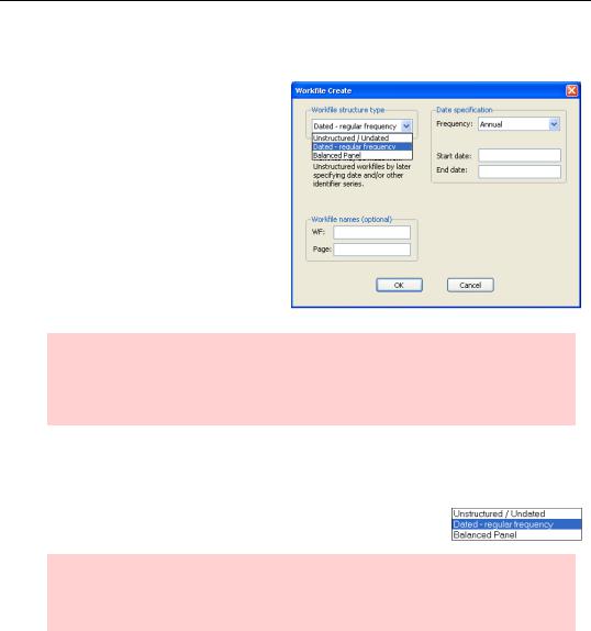
Open EViews and use the menu to choose File/New/Workfile… The Workfile Create dialog pops up.
Hint: Alternatively, you can type
wfcreate
in the command pane to bring up the same dialog.
You’ll notice in the dialog that EViews defaults to “Dated – regular frequency” and “Annual.” However, the data shown in Table 1: Academic Salary Data Excerpt are just numbered sequentially. They aren’t dated.
Choosing the Workfile structure type dropdown menu offers three choices:
Hint: Changing the type of workfile structure can be mildly inconvenient, so it pays to think a little about this decision. In contrast, simply increasing or decreasing the range of observations in the workfile is quite easy.
Our data are Unstructured/Undated. Select this option. Later in this chapter we’ll discuss Dated – regular frequency. (Balanced Panel is deferred to Chapter 11, “Panel—What’s My Line?.”)
26—Chapter 2. EViews—Meet Data
Hint: Alternatively, we can enter
wfcreate u
in the command pane.
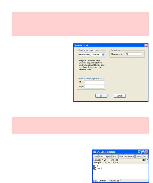
Unstructured/Undated instructs EViews to number the observations from 1 through however-many-obser- vations-you-have. In our example we have 28 observations. Enter “28” in the field marked “Observations:” If you’d like to give your workfile a name you can enter the name in the “WF:” field at the lower right. You can also name the workfile when you save it, so giving a name now or later is purely a matter of personal preference.
Hit  and the workfile is created for you.
Hint: If you like, the workfile can be created with the single command
wfcreate u 28
Deconstructing the Workfile
There’s no data yet, but let’s dissect what EViews starts you off with. The initial workfile window looks something like the picture to the right.
The title bar shows the name of the workfile. Since we didn’t enter a name for the workfile in the dialog, EViews uses “UNTITLED” in the title bar.
The workfile window has buttons at the top and
tabs at the bottom. The buttons provide menus linked to each EViews window type. The tabs mark pages, essentially workfiles within a workfile. We’ll come back to pages in Chapter 9, “Page After Page After Page”; they’re particularly useful for holding sets of data with different indices.