
- •Table of Contents
- •Foreword
- •Chapter 1. A Quick Walk Through
- •Workfile: The Basic EViews Document
- •Viewing an individual series
- •Looking at different samples
- •Generating a new series
- •Looking at a pair of series together
- •Estimating your first regression in EViews
- •Saving your work
- •Forecasting
- •What’s Ahead
- •Chapter 2. EViews—Meet Data
- •The Structure of Data and the Structure of a Workfile
- •Creating a New Workfile
- •Deconstructing the Workfile
- •Time to Type
- •Identity Noncrisis
- •Dated Series
- •The Import Business
- •Adding Data To An Existing Workfile—Or, Being Rectangular Doesn’t Mean Being Inflexible
- •Among the Missing
- •Quick Review
- •Appendix: Having A Good Time With Your Date
- •Chapter 3. Getting the Most from Least Squares
- •A First Regression
- •The Really Important Regression Results
- •The Pretty Important (But Not So Important As the Last Section’s) Regression Results
- •A Multiple Regression Is Simple Too
- •Hypothesis Testing
- •Representing
- •What’s Left After You’ve Gotten the Most Out of Least Squares
- •Quick Review
- •Chapter 4. Data—The Transformational Experience
- •Your Basic Elementary Algebra
- •Simple Sample Says
- •Data Types Plain and Fancy
- •Numbers and Letters
- •Can We Have A Date?
- •What Are Your Values?
- •Relative Exotica
- •Quick Review
- •Chapter 5. Picture This!
- •A Simple Soup-To-Nuts Graphing Example
- •A Graphic Description of the Creative Process
- •Picture One Series
- •Group Graphics
- •Let’s Look At This From Another Angle
- •To Summarize
- •Categorical Graphs
- •Togetherness of the Second Sort
- •Quick Review and Look Ahead
- •Chapter 6. Intimacy With Graphic Objects
- •To Freeze Or Not To Freeze Redux
- •A Touch of Text
- •Shady Areas and No-Worry Lines
- •Templates for Success
- •Point Me The Way
- •Your Data Another Sorta Way
- •Give A Graph A Fair Break
- •Options, Options, Options
- •Quick Review?
- •Chapter 7. Look At Your Data
- •Sorting Things Out
- •Describing Series—Just The Facts Please
- •Describing Series—Picturing the Distribution
- •Tests On Series
- •Describing Groups—Just the Facts—Putting It Together
- •Chapter 8. Forecasting
- •Just Push the Forecast Button
- •Theory of Forecasting
- •Dynamic Versus Static Forecasting
- •Sample Forecast Samples
- •Facing the Unknown
- •Forecast Evaluation
- •Forecasting Beneath the Surface
- •Quick Review—Forecasting
- •Chapter 9. Page After Page After Page
- •Pages Are Easy To Reach
- •Creating New Pages
- •Renaming, Deleting, and Saving Pages
- •Multi-Page Workfiles—The Most Basic Motivation
- •Multiple Frequencies—Multiple Pages
- •Links—The Live Connection
- •Unlinking
- •Have A Match?
- •Matching When The Identifiers Are Really Different
- •Contracted Data
- •Expanded Data
- •Having Contractions
- •Two Hints and A GotchYa
- •Quick Review
- •Chapter 10. Prelude to Panel and Pool
- •Pooled or Paneled Population
- •Nuances
- •So What Are the Benefits of Using Pools and Panels?
- •Quick (P)review
- •Chapter 11. Panel—What’s My Line?
- •What’s So Nifty About Panel Data?
- •Setting Up Panel Data
- •Panel Estimation
- •Pretty Panel Pictures
- •More Panel Estimation Techniques
- •One Dimensional Two-Dimensional Panels
- •Fixed Effects With and Without the Social Contrivance of Panel Structure
- •Quick Review—Panel
- •Chapter 12. Everyone Into the Pool
- •Getting Your Feet Wet
- •Playing in the Pool—Data
- •Getting Out of the Pool
- •More Pool Estimation
- •Getting Data In and Out of the Pool
- •Quick Review—Pools
- •Chapter 13. Serial Correlation—Friend or Foe?
- •Visual Checks
- •Testing for Serial Correlation
- •More General Patterns of Serial Correlation
- •Correcting for Serial Correlation
- •Forecasting
- •ARMA and ARIMA Models
- •Quick Review
- •Chapter 14. A Taste of Advanced Estimation
- •Weighted Least Squares
- •Heteroskedasticity
- •Nonlinear Least Squares
- •Generalized Method of Moments
- •Limited Dependent Variables
- •ARCH, etc.
- •Maximum Likelihood—Rolling Your Own
- •System Estimation
- •Vector Autoregressions—VAR
- •Quick Review?
- •Chapter 15. Super Models
- •Your First Homework—Bam, Taken Up A Notch!
- •Looking At Model Solutions
- •More Model Information
- •Your Second Homework
- •Simulating VARs
- •Rich Super Models
- •Quick Review
- •Chapter 16. Get With the Program
- •I Want To Do It Over and Over Again
- •You Want To Have An Argument
- •Program Variables
- •Loopy
- •Other Program Controls
- •A Rolling Example
- •Quick Review
- •Appendix: Sample Programs
- •Chapter 17. Odds and Ends
- •How Much Data Can EViews Handle?
- •How Long Does It Take To Compute An Estimate?
- •Freeze!
- •A Comment On Tables
- •Saving Tables and Almost Tables
- •Saving Graphs and Almost Graphs
- •Unsubtle Redirection
- •Objects and Commands
- •Workfile Backups
- •Updates—A Small Thing
- •Updates—A Big Thing
- •Ready To Take A Break?
- •Help!
- •Odd Ending
- •Chapter 18. Optional Ending
- •Required Options
- •Option-al Recommendations
- •More Detailed Options
- •Window Behavior
- •Font Options
- •Frequency Conversion
- •Alpha Truncation
- •Spreadsheet Defaults
- •Workfile Storage Defaults
- •Estimation Defaults
- •File Locations
- •Graphics Defaults
- •Quick Review
- •Index
- •Symbols

374—Chapter 15. Super Models
Numerical accuracy
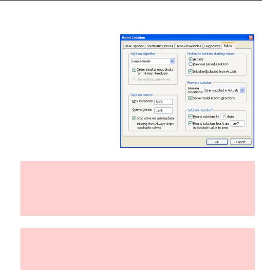
Computers aren’t nearly so bright as your average junior high school student, so they use numerical methods which come up with approximate solutions. If you’d like a “more accurate” answer, you need to tell EViews to be more fussy. Click and choose the
Solver tab. Change Convergence to “1e-09”, to get that one extra digit of accuracy.
Vanity hint: In the problem at hand, all we’re doing is making the answer look pretty.
In more complicated problems a smaller convergence limit has the advantage that it helps assure that the computer reaches the right answer. The disadvantages are that the solution takes longer, and that sometimes if you ask for extreme accuracy no satisfactory answer can be found.
Accurately understanding accuracy: Don’t confuse numerical accuracy with model accuracy. The solver options control numerical accuracy. These options have nothing to do with the accuracy of your model or your data. The latter two are far more important. Unfortunately, you can’t improve model or data accuracy by clicking on a button.
Your Second Homework
Odds are that your second homework assignment in your first introductory macroeconomics class asked what would happen to GDP if G were to rise. In other words, how do the results of this new scenario differ from the baseline results?

Your Second Homework—375
Making Scenarios
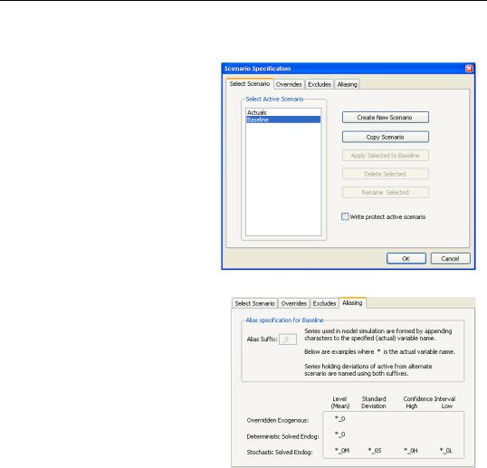
EViews puts a single set of assumptions about the inputs to a model together with the resulting solution in a scenario. The solutions based on the original data are called the Baseline. So the solutions to our first homework problem are stored in the baseline scenario. Choosing Scenarios… from the View menu brings up the
Scenario Specification dialog with the Select Scenario tab showing. The Baseline scenario that’s showing was automatically created when we solved the model.
A look at the aliasing tab shows that the suffix for Baseline results is “_0.” The fields are greyed out because EViews assigns the suffix for the Baseline.

376—Chapter 15. Super Models
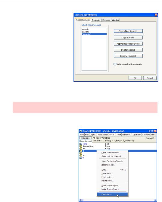
We want to ask what would happen in a world in which government spending were 10 (billion dollars) higher than it was in the real world. This is a new scenario, so click on the Select Scenario tab. Scenario 1 is associated with the alias “_1”. If you like, you can rename the new scenario to something more meaningful or change the suffix, but we’ll just click
for now.
We want to instruct EViews to use different values of G in this scenario. We’ll create the series G_1 with the command:
series g_1 = g + 10
Hint: We chose the name “G_1” because the suffix has to match the scenario alias.
Overriding Baseline Data
Back in the model window click
and then right-click on G and choose Properties….

Your Second Homework—377
On the Properties dialog, check Use override in series in scenario to instruct EViews to substitute G_1 for G.
Now .
Hint: You can override an exogenous variable but you cannot override an endogenous variable because the latter would require a change to the structure of the model.
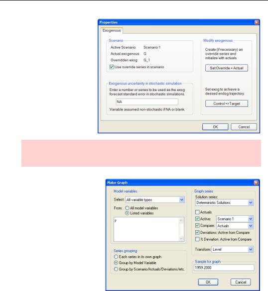
New series Y_1 and CONS_1 appear in the workfile. Return to Proc/Make Graph… in the model window, choose Listed Variables, list Y, and check Compare. As you can see in the dialog, many options are available. We’re asking for a comparison of the baseline solution to the new scenario. We can show the difference between the two— by checking one of the Deviations boxes—in either units or as a percentage.