

Vector Autoregressions—VAR—361
The answer, which is unsurprising given the reported coefficients and standard errors, is “No, the coefficients are not equal.”
Vector Autoregressions—VAR
In Chapter 8, “Forecasting,” we discussed predictions based on ARMA and ARIMA models. This kind of forecasting generalizes, at least in the case of autoregressive models, to multiple dependent variables through the use of vector autoregressions or VARs. While VARs can be quite sophisticated (see the User’s Guide), at its heart a VAR simply takes a list of series and regresses each on its own past values as well as lags of all the other series in the list.
Create a VAR object either through the Object menu or the var command. The  button opens the VAR Specification dialog. Enter the variables to be explained in the Endogenous Variables field.
362—Chapter 14. A Taste of Advanced Estimation
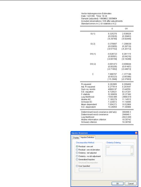
EViews estimates least squares equations for both series.
Impulse response
To answer the question “How do the series evolve following a shock to the error term?” click the  button. The phrase “following a shock” is less straightforward than it sounds. In general, the error terms will be correlated across equations, so one wants to be careful about shocking one equation but not the other. And how big a shock? One unit? One standard deviation?
You control how you deal with these questions on the Impulse Definition tab. For illustration purposes, let’s consider a unit shock to each error term.
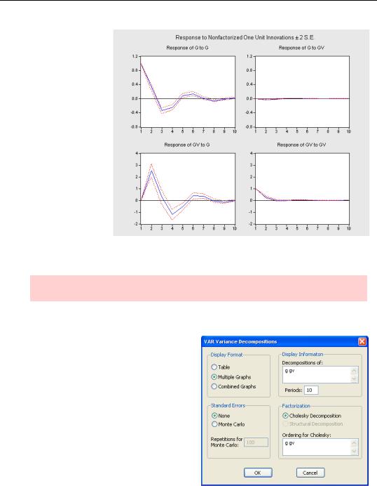
Once we choose a specification, we get a set of impulse response functions. We get a plot of the response over time of each endogenous variable to a shock in each equation. In other words, we see how G responds to shocks to both the G equation and the GV equation, and similarly, how GV responds to shocks to the GV equation and the G equation.
Vector Autoregressions—VAR—363
By default (there are other options) we get one figure containing all four impulse response graphs. The line graph in the upper left-hand corner shows that following a shock to the G equation, G wiggles around for a quarter or so, but by the fifth quarter the response has effectively dissipated. In contrast, the upper righthand corner graph shows that G is
effectively unresponsive to shocks in the GV equation.
Hint: The dashed lines enclose intervals of plus or minus two standard errors.
Variance decomposition
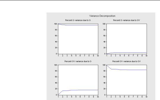
How much of the variance in G is explained by shocks in the G equation and how much is explained by shocks in the GV equation? The answer depends on, among other things, the estimated coefficients, the estimated standard error of each equation, and the order in which you evaluate the shocks. View/Variance Decomposition… leads to the VAR Variance Decompositions dialog where you can set various options.
364—Chapter 14. A Taste of Advanced Estimation
The variance decomposition shows one graph for the variance of each equation from each source. The horizontal axis tells the number of periods following a shock to which the decomposition applies and the vertical axis gives the fraction of variance explained by the shock source. In this example, most of the variance comes from
the “own-shock” (i.e., G-shocks effect on G), rather than from the shock to the other equation.
Forecasting from VARs
In order to forecast from a VAR, you need to use the model object. An example is given in Simulating VARs in Chapter 15, “Super Models.”
Vector error correction, cointegration tests, structural VARs
VARs have become an important tool of modern econometrics, especially in macroeconomics. Since the User’s Guide devotes an entire chapter to the subject, we’ll just say that the VAR object provides tools that handle everything listed in the topic heading above this paragraph.
Quick Review?
A quick review of EViews’ advanced estimation features suggests that a year or two of Ph.D.-level econometrics would help in learning to use all the available tools. This chapter has tried to touch the surface of many of EViews advanced techniques. Even this extended introduction hasn’t covered everything that’s available. For example, EViews offers a sophisticated state-space (Kalman filter) module. As usual, we’ll refer you to the User’s Guide for more advanced discussion.