

Maximum Likelihood—Rolling Your Own—355
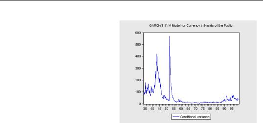
Is the 0.014 estimated GARCH-M coefficient large? Again, we look at the conditional variance using the Garch Graph menu item. In a few periods, the conditional variance reaches 400 to 500, so the structural effect is on the order of 6 or 7 (the estimated coefficient multiplied by the estimated conditional variance.) That’s larger than several of the monthly dummies. But for most of the sample, the GARCH-M effect is relatively small.
Maximum Likelihood—Rolling Your Own
Despite EViews’ extensive selection of estimation techniques, sometimes you want to custom craft your own. EViews provides a framework for customized maximum likelihood estimation (mle). The division of labor is that you provide a formula defining the contribution an observation makes to the likelihood function, and EViews will produce estimates and the expected set of associated statistics. For an example, we’ll return to the weighted least squares problem which opened the chapter. This time, we’ll estimate the variances and coefficients jointly.
Our first step is to create a new LogL object, using either the Object/New Object… menu or a command like:
logl weighted_example
Opening  brings up a text area for entering definitions. Think of the commands here as a series of series commands—only without the command name series being given—that EViews will execute in sequential order. These commands build up the definition of the contribution to the likelihood function. The file also includes one line with the keyword @logl, which identifies which series holds the contribution to the likelihood function.
356—Chapter 14. A Taste of Advanced Estimation
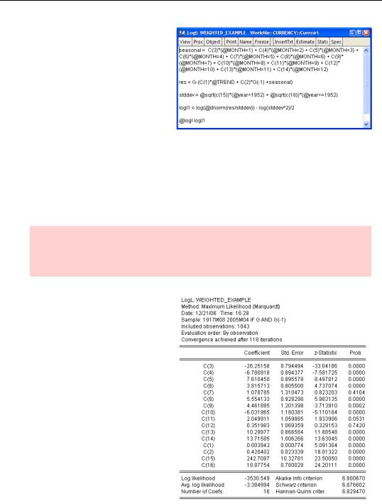
Let’s take apart our example specification shown to the right. We broke the definition of the error term into two parts simply because it was easier to type. The first equation defines the seasonal component. The second equation is the difference between observed currency growth and predicted currency growth. The third equation defines
the error term standard deviation as coming from either the early-period variance, C(15), or the late-period variance, C(16). Note that all these definitions depend on the values in the coefficient vector C, and will change as EViews tries out new coefficient values.
The fourth line defines LOGL1, which gives the contribution to the log likelihood function, assuming that the errors are distributed independent Normal. The last line announces to EViews that the contributions are, in fact, in LOGL1.
Hint: We didn’t really type in that long seasonal component. We copied it from the representations view of the earlier least squares results, pasted, and did a little judicious editing.
The maximum likelihood coefficients are close to the coefficients estimated previously. We’ve gained formal estimates of the variances, along with standard errors of the variance estimates.
The User’s Guide devotes an entire chapter to the ins and outs of maximum likelihood estimation. Additionally, EViews ships with over a dozen files illustrating definitions of likelihood functions across a wide range of examples.
System Estimation—357
Hint: Unlike nearly all other EViews estimation procedures, maximum likelihood won’t deal with missing data. The series defined by @logl must be available for every observation in the sample. Define an appropriate sample in the Estimation dialog. If you accidentally include missing data, EViews will give an error message identifying the offending observation.
System Estimation
So far, all of our estimation has been of the one-equation-at-a-time variety. System estimation, in contrast, estimates jointly the parameters of two or more equations. System estimation offers three econometric advantages, at the cost of one disadvantage. The first plus is that a parameter can appear in more than one equation. The second plus is that you can take advantage of correlation between error terms in different equations. The third advantage is that cross-equation hypotheses are easily tested. The disadvantage is that if one equation is misspecified, that misspecification will pollute the estimation of all the other equations in the system.
Worthy of repetition hint: If you want an estimated coefficient to have the same value in more than one equation, system estimation is the only way to go. Use the same coefficient name and number, e.g., C(3), in each equation you specify. The jargon for this is “constraining the coefficients.” Note that you can constrain some coefficients across equations and not constrain others.
To create a system object either give the system command or use the menu
Object/New Object…. Enter one or more equation specifications in the text area.
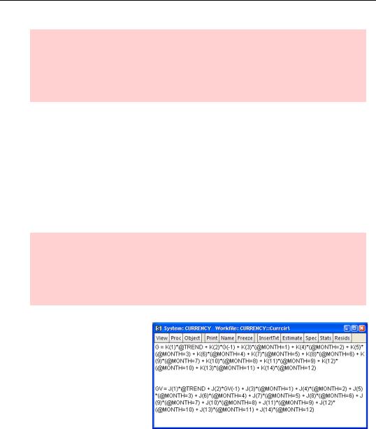
We’ve added data on the growth in bank vault cash, GV, to our data set on growth in currency in the hands of the public, G. The specifica-
tion shown is identical for both cash components.
358—Chapter 14. A Taste of Advanced Estimation
Hint: It helped to copy-and-paste from the representations view of the earlier least squares results, and then to use Edit/Replace to change the coefficients from “C” to “K” and “J.”
Before we can estimate the system shown, we need to create the coefficient vectors K and J. That can be done with the following two commands given in the command pane, not in the system window:
coef(14) j
coef(14) k
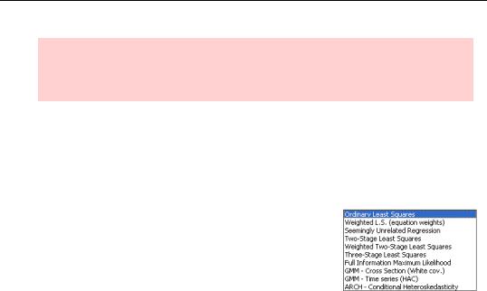
EViews provides a long list of estimation methods which can be applied to a system. Click the  button to bring up the System Estimation dialog and then choose an estimation method from the Method dropdown.
System Estimation—359
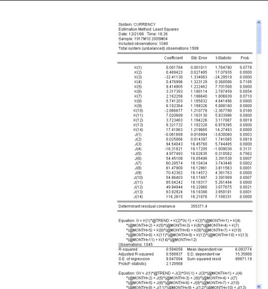
Choosing Ordinary Least Squares produces estimates for both equations. (The output is long; only part is shown here.) Note that the results for currency in the hands of the public are precisely the same as those we saw previously. We asked for equation-by-equation ordinary least squares, and that’s what we got—the equivalent of a bunch of ls commands.
360—Chapter 14. A Taste of Advanced Estimation
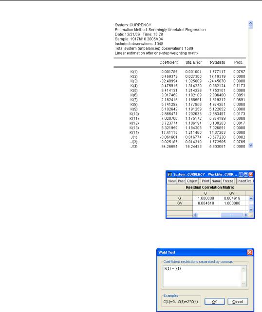
Instead of equation-by-equa- tion least squares, we might try a true systems estimator, such as seemingly unrelated regressions (SUR). The upper portion of the SUR results is shown to the right.
The estimated coefficients haven’t changed much in this example. The difference between the two estimates is that the latter accounts for correlation between the two equations, while the former doesn’t. The Residuals/Correlation Matrix view shows the estimated cross-equation correlation. In this case, there is very little correlation—that’s why the SUR estimates came out about the same the estimates from equation-by-equation least squares.
Because coefficient estimates from all the equations are made jointly, cross-equation hypotheses are easily tested. For example, to check the hypothesis that the coefficients on trend are equal for cash in the hands of the public and vault cash, choose View/Coefficient Diagnostics/Wald Coefficient Tests… and fill out the
Wald Test dialog in the usual way.