

Generalized Method of Moments—347
Thus, to get 2SLS results we can give the command:
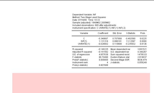
tsls inf c inf(1) unrate(-1) @ c unrate(-1) inf(-1) inf(-2)
The coefficient on future inflation is now close to 1.0, as theory predicts. The coefficient on unemployment is negative, albeit small and not significant.
Hint: By default, if you don’t include the constant, C, in the instrument list, EViews puts one in for you. You can tell EViews not to add the constant by unchecking the Include a constant box in the estimation dialog.
Did you notice the R2 in the 2SLS output? It’s negative. This means that the equation fits the data really poorly. That’s okay. Our interest here is in accurate parameter estimation.
Generalized Method of Moments
What happens if you put together nonlinear estimation and two-stage least squares? While EViews will happily estimate a nonlinear equation using the tsls command, nowadays econometricians are more likely to use the Generalized Method of Moments, or GMM.
Two-stage least squares can be thought of as a special case of GMM. GMM extends 2SLS in two dimensions:
•GMM estimation typically accounts for heteroskedasticity and/or serial correlation.
•GMM specification is based on an orthogonality condition between a (possibly nonlinear) function and instruments.
As an example, suppose instead of the tsls command above we gave the gmm command:
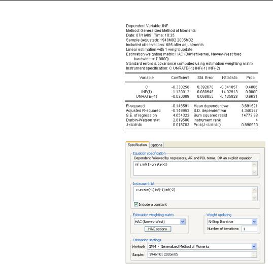
gmm inf c inf(1) unrate(-1) @ c unrate(-1) inf(-1) inf(-2)
348—Chapter 14. A Taste of Advanced Estimation
The resulting estimate is close to the 2SLS estimate, but it’s not identical. By default, EViews applies one of the many available options for estimation that is robust to heteroskedasticity and serial correlation.
Clicking the  button reveals the GMM Specification tab. The entire right side of this tab is devoted to the choice of robust estimation methods. See the User’s Guide for more information.
Orthogonality Conditions
The basic notion behind GMM is that each of the instruments is orthogonal to a specified function. You can specify the function in any of three ways:
•If you give the usual—dependent variable followed by independent variables—series list, the function is the residual.
•If you give an explicit equation, linear or nonlinear, the function is the value to the left of the equal sign minus the value to the right of the equal sign.
•If you give a formula with no equal sign, the formula is the function.
See System Estimation, below, for a brief discussion of GMM estimation for systems of equations.
Limited Dependent Variables—349
Limited Dependent Variables
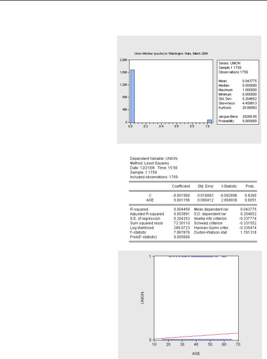
Suppose we’re interested in studying the determinants of union membership and that, coincidentally, we have data on a cross-section of workers in Washington State in the workfile “CPSMAR2004WA.wf1”. The series UNION is coded as one for union members and zero for non-members. Between four and five percent of workers in our sample are members of a union.
Is age an important determinant
of union membership? We might run a regression to see. According to the least squares results, age is highly significant statistically (the t-statistic is 2.8), but doesn’t explain much of the variation in the dependent variable (the R2 is low).
We can also look at the regression on a scatter plot. The dependent variable is all zeros and ones. The predicted values from the regression lie on a continuous line.
While the regression results aren’t necessarily “wrong,” what does it mean to say that predicted union membership is 0.045? Either you are a member of a union, or you are not a member of a union!
This example is a member of a class called limited dependent
350—Chapter 14. A Taste of Advanced Estimation
variable problems. EViews provides estimation methods for binary dependent variables, as in our union membership example, ordered choice models, censored and truncated models (tobit being an example), and count models. The User’s Guide provides its usual clear explanation of how to use these models in EViews, as well as a guide to the underlying theory.
We’ll illustrate with the simplest model: logit.
Logit
Instead of fitting zeros and ones, the logit model uses the right-hand side variables to predict the probability of being a union member, i.e., of observing a 1.0. One can think of the model as having two parts. First, an index s is created, which is a weighted combination of the explanatory variables. Then the probability of observing the outcome depends on the cumulative distribution function (cdf) of the index. Logit uses the cdf of the logistic distribution; probit uses the normal distribution instead.
The logit command is straightforward:
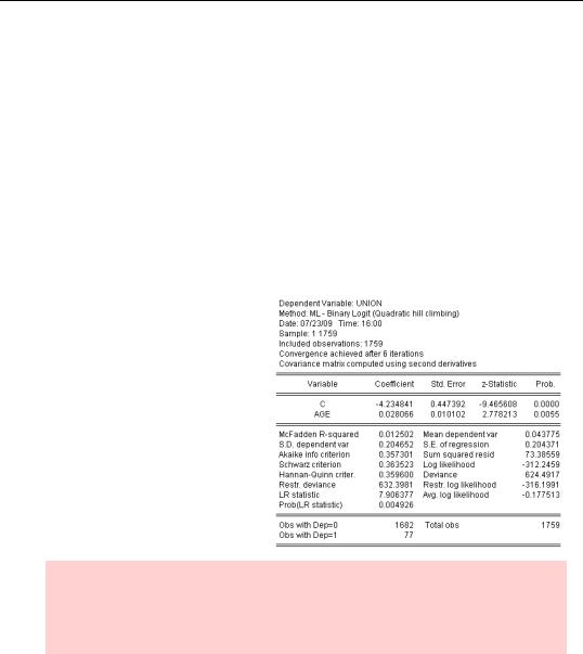
logit union c age
The coefficients shown in the output are the coefficients for constructing the index. In this case, our estimated model says:
s = – 4.23 + 0.028 × age prob(union= 1) = 1 – F(–s)
F(s)= es ⁄ (1 + es)
Textbook hint: Textbooks usually describe the relation between probability and index in a logit with prob(union= 1)= F(s) rather than
prob(union= 1)= 1 – F(–s) . The two are equivalent for a logit (or a probit), but differ for some other models.