

Nonlinear Least Squares—341
Nonlinear Least Squares
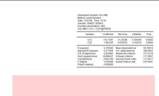
Much as Molière’s bourgeois gentilhomme was pleased to discover he had been speaking prose all his life, you may be happy to know that in using the ls command you’ve been doing nonlinear estimation all along! Here’s a very simple estimate of trend NYSE volume growth from the data set “NYSEVolume.wf1”:
ls volume c @trend
Switch to the Representations view
and look at the section titled “Estimation Equation.” The least squares command
orders estimation of the equation volume = a + b × @trend , except that
since EViews doesn’t display Greek letters, C(1) is used for a and C(2) is used for b .
If you double-click on  you’ll see that the
first two elements of C equal the just-estimated coefficients. In fact, every time EViews estimates an equation it stores the results in the vector C.
Hint: It may look curious that C(1), C(2), etc. seem to be labeled R1, R2, and so on. R1 and R2 are generic labels for row 1 and row 2 in a coefficient vector. The same setup is used generally for displaying vectors and matrices.
The key to nonlinear estimation is:
• Feed the ls command a formula in place of a list of series.
If you enter the command:
ls volume = c(1) + c(2)*@trend
342—Chapter 14. A Taste of Advanced Estimation
you get precisely the same results as above. The only difference is that the formula in the command is reported in the top panel and that C(1) and C(2) appear in place of series names.
Hint: Unlike series where a number in parentheses indicates a lead or lag, the number following a coefficient is the coefficient number. C(1) is the first element of C, C(2) is the second element of C, and so on.
Naming Your Coefficients
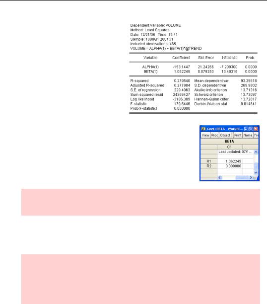
Least squares with a series list always stores the estimated coefficients in C, but you’re free to create other coefficient vectors and use those coefficients when you specify a formula. To create a coefficient vector, give the command coef(n) newname, replacing n with the desired length of the coefficient vector and newname with the vector’s name. Here’s an example:
coef(1) alpha
coef(2) beta
ls volume = alpha(1) + beta(1)*@trend
Nonlinear Least Squares—343
The results haven’t changed, but the names given to the estimated coefficients have. As a side effect, the results are stored in ALPHA and BETA, not in C.
Notice that the slope coefficient has
been stored in BETA(1), and that since we didn’t reference BETA(2) nothing has been stored in it.
Hint: Since every new estimate specified with a series list replaces the values in C, it makes sense to use a different coefficient vector for values you’d like to keep around.
Coefficient vectors aren’t just for storing results. They can also be used in computations. For example, to compute squared residuals one could type:
series squared_residuals=(volume-alpha(1)-beta(1)*@trend)^2
Hint: It would, of course, been easier in this example to enter:
series squared_residuals=resid^2
But then we wouldn’t have had the opportunity to demonstrate how to use coefficients in a computation.
344—Chapter 14. A Taste of Advanced Estimation
Making It Really Nonlinear
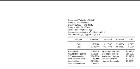
To estimate a nonlinear regression, enter a nonlinear formula in the ls
command. For example, to estimate the equation volume = atb use
the command:
ls volume = c(1)*(1+@trend)^c(2)
Notice the big improvement in R2 over the linear model.
You can place most any nonlinear formula you like on the right hand side of the equation.
If you’re lucky, getting a nonlinear estimate is no harder than getting a linear estimate. Sometimes, though, you’re not lucky. While EViews uses the standard closed-form expression for finding coefficients for linear models, nonlinear models require a search procedure. The line in the top panel “Convergence achieved after 108 iterations” indicates that EViews tried 108 sets of coefficients before settling on the ones it reported. Sometimes no satisfactory estimate can be found. Here are some tricks that may help.
Re-write the formula
Notice we actually estimated volume = a(1 + t)b instead of volume = atb . Why? The first value of @TREND is zero, and in this particular case EViews had difficulty raising 0 to a power. This very small re-write got around the problem without changing anything substantive. Sometimes one expression of a particular functional form works when a different expression of the same function doesn’t.
Fiddle with starting values
EViews begins its search with whatever values happen to be sitting in C. Sometimes a search starting at one set of values succeeds when a search at different values fails. If you have good guesses as to the true values, use those guesses for a starting point. One way to change starting values is to double-click on  and edit in the usual way. You can also use the param statement to change several coefficient values at once, as in:
param c(1) 3.14159 c(2) 2.718281828
2SLS—345
Change iteration limits
If the estimate runs but doesn’t converge, give the same command again. Since EViews stores the last estimated coefficients in C, the second estimation run picks up exactly where the first one left off.
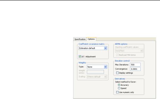
Alternatively, click the  button and switch to the Options tab. Try increasing Max iterations. You can also put a larger number in the Convergence field, if you’re willing to accept potentially less accurate answers.
2SLS
For consistent parameter estimation, the sine non qua assumption of least squares is that the error
terms are uncorrelated with the right hand side variables. When this assumption fails, econometricians turn to two-stage least squares, or 2SLS, a member of the instrumental variable, or IV, family. 2SLS augments the information in the equation specification with a list of instruments—series that the econometrician believes to be correlated with the right-hand side variables and uncorrelated with the error term.
As an example, consider estimation of the “new Keynesian Phillips curve,” in which inflation depends on expected future inflation and unemployment—possibly lagged. In the fol-
lowing oversimplified specification,
pt = a + bpet + 1 + gunt – 1
346—Chapter 14. A Taste of Advanced Estimation
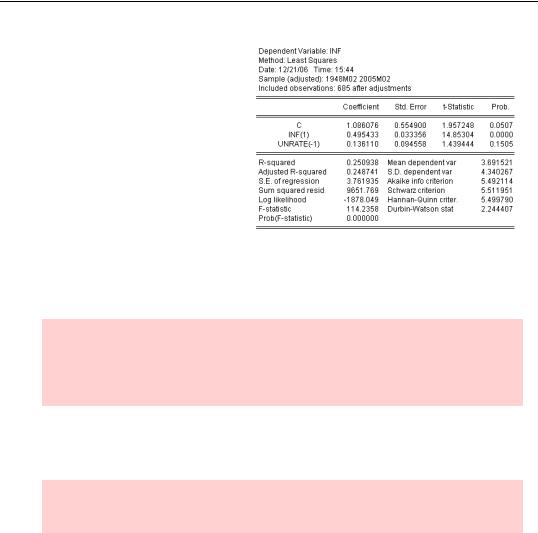
we expect b ≈ 1 and g < 0 . Using monthly U.S. data in “CPI_AND_UNEMPLOYMENT.wf1”, we could try to estimate this equation by least squares with the command:
ls inf c inf(1) unrate(-1)
Notice that the estimated coefficients are very different from the coefficients predicted by theory. The coefficient on future inflation is approximately 0.5, rather than 1.0,
and the coefficient on unemployment is positive. The econometric difficulty is that by using actual future inflation as a proxy for expected future inflation, we introduce an “errors-in- variables” problem. We’ll try a 2SLS estimate, using lagged information as instruments.
Econometric digression: If a right-hand side variable in a regression is measured with random error, the equation is said to suffer from errors-in-variables. Errors-in-variables leads to biased coefficients in ordinary least squares. Sometimes this can be fixed with 2SLS.
The 2SLS command uses the same equation specification as does least squares. The equation specification is followed by an “@” and the list of instruments. The command name is tsls.
Hint: It’s tsls rather than 2sls because the convention is that computer commands start with a letter rather than a number.