

Chapter 14. A Taste of Advanced Estimation
Estimation is econometric software’s raison d’être. This chapter presents a quick taste of some of the many techniques built into EViews. We’re not going to explore all the nuanced variations. If you find an interesting flavor, visit the User’s Guide for in-depth discussion.
Weighted Least Squares
Ordinary least squares attaches equal weight to each observation. Sometimes you want certain observations to count more than others. One reason for weighting is to make sub-popu- lation proportions in your sample mimic sub-population proportions in the overall population. Another reason for weighting is to downweight high error variance observations. The version of least squares that attaches weights to each observation is conveniently named weighted least squares, or WLS.
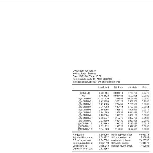
In Chapter 8, “Forecasting” we looked at the growth of currency in the hands of the public, estimating the equation shown here. We used ordinary least squares for an estimation technique, but you may remember that the residuals were much noisier early in the sample than they were later on. We might get a better estimate by giving less weight to the early observations.
336—Chapter 14. A Taste of Advanced Estimation
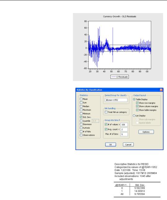
As a rough and ready adjustment after looking at the residual plot, we’ll choose to give more weight to observations from 1952 on and less to those earlier.
We used a Stats By Classification… view of RESID to find error standard deviations for each subperiod.
You can see that the residual standard deviation falls in half from 1952. We’ll use this information to create a series, ROUGH_W, for weighting observations:
series rough_w = 14*(@year<1952) + 6*(@year>=1952)
That’s the heart of the trick in instructing EViews to do weighted least squares—you need to create a series which holds the weight for every observation. When performing weighted least squares using the default settings,
EViews then multiplies each observation by the weight you supply. Essentially, this is equivalent to replicating each observation in proportion to its weight.
Weighted Least Squares—337
Hint: In fact, if the weight is wi , the EViews default scaling multiplies the data by wi ⁄ w —the observation weight divided by the mean weight. In theory this makes no difference, but sometimes the denominator helps with numerical computation issues.
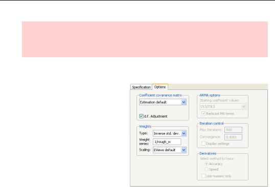
The Weighted Option
Open the least squares equation EQ01 in the workfile, click the  button, and switch to the Options tab. In the Weights groupbox, select Inverse std.dev. from the Type dropdown and enter the weight series in the Weight series field. Notice that we’ve entered 1/ROUGH_W. That’s because 1/ROUGH_W is roughly proportional to the inverse of the error standard deviation. As is generally true in EViews, you can enter an expression wherever a series is called for.
338—Chapter 14. A Taste of Advanced Estimation
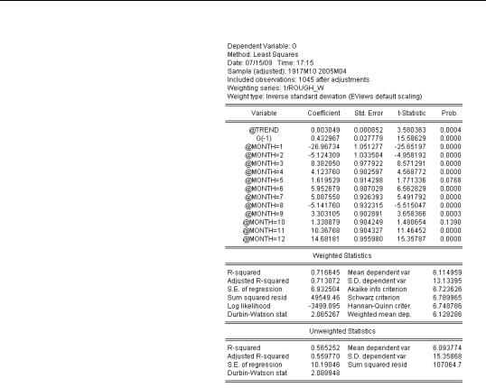
The weighted least squares estimates include two summary statistics panels. The first panel is calculated from the residuals from the weighted regression, while the second is based on unweighted residuals. Notice that the unweighted R2 from weighted least squares is a little lower than
reported in the original ordinary least squares estimate, just as it should be.
Heteroskedasticity
One of the statistical assumptions underneath ordinary least squares is that the error terms for all observations have a common variance; that they are homoskedastic. Vary-
ing variance errors are said, in contrast, to be heteroskedastic. EViews offers both tests for heteroskedasticity and methods for producing correct standard errors in the presence of heteroskedasticity.
Heteroskedasticity—339
Tests for Heteroskedastic Residuals
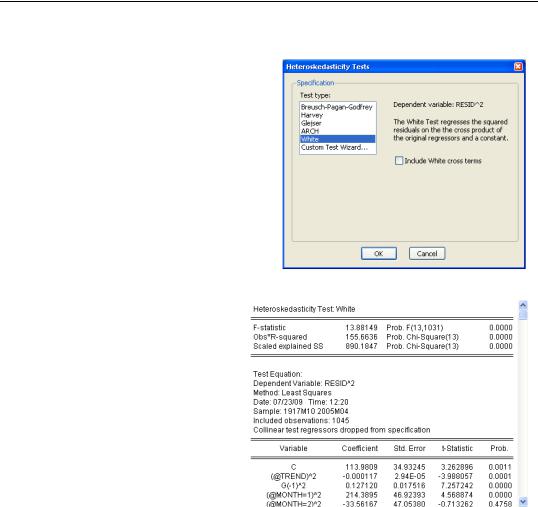
The Residual Diagnostics/Heteroskedasticity Tests... view of an equation offers variance heteroskedasticity tests, including two variants of the White heteroskedasticity test. The White test is essentially a test of whether values of the right-hand side variables—and/or their cross terms, x21, x1 × x2, x22 , etc.—help explain the squared residuals. To perform a White test with only the squared terms (no cross terms), you should uncheck the Include White cross terms box.
Here are the results of the White test (without cross terms) on our currency growth equation. The F- and x2- statistics reported in the top panel decisively reject the null hypothesis of homoskedasticity.
The bottom panel— only part of which is shown—shows the auxiliary regression used to compute the test statistics.
340—Chapter 14. A Taste of Advanced Estimation
Heteroskedasticity Robust Standard Errors
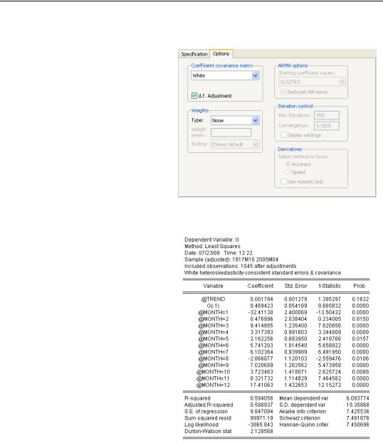
One approach to dealing with heteroskedasticity is to weight observations such that the weighted data are homoskedastic. That’s essentially what we did in the previous section. A different approach is to stick with least squares estimation, but to correct standard errors to account for heteroskedasticity. Click the  button in the equation window and switch to the Options tab. Select either White or HAC (Newey-West) in the dropdown in the Coefficient covariance matrix
group. As an example, we’ll trumpet the White results.
Compare the results here to the least squares results shown on page 335. The coefficients, as well as the summary panel at the bottom, are identical. This reinforces the point that we’re still doing a least squares estimation, but adjusting the standard errors.
The reported t-statistics and p-values reflect the adjusted standard errors. Some are smaller than before and some are larger. Hypothesis tests computed using Coefficient Diag- nostics/Wald-Coefficient Restrictions… correctly account for the adjusted standard errors. The Omitted Variables and Redundant Variables tests do not use the adjusted standard errors.