


18—Chapter 1. A Quick Walk Through
Saving your work
Quite satisfactory, but this is getting to be thirsty work. Before we take a break, let’s save our equation in the workfile. Hit the  button on the equation window. In the upper field type a meaningful name.
Hint: Spaces aren’t allowed when naming an object in EViews.
Prior to this step the title bar of the equation window read “Equation: untitled.” Using the  button changed two things: the equation now has a name which appears in the title bar, and more importantly, the equation object is stored in the workfile. You can see these
changes below. If you like, close the equation window and then double-click on  to re-open the equation. But don’t take the break quite yet!

Saving your work—19
Before leaving the computer, click on the workfile window. Use the File menu choice File/Save As… to save the workfile on the disk.
Now would be a good time to take a break. In fact, take a few minutes and indulge in your favorite beverage.
Back so soon? If your computer froze while you were gone you can start up EViews and use File/Open/EViews Workfile… to reload the workfile you saved before the break.
Your computer didn’t freeze, did it? (But then, you probably didn’t really take a break either.) This is the spot in which authors enjoin you to save your work often. The truth is, EViews is remarkably stable software. It certainly crashes less often than your typical word processor. So, yes, you should save your workfile to disk as a safety measure since it’s easy, but there’s a different reason that we’re emphasizing saving your workfile.
EViews doesn’t have an Undo feature.
As you work you make changes to the data in the workfile. Sometimes you find you’ve gone up a blind alley and would like to back out. Since there is no Undo feature, we have to substitute by doing Save As… frequently. If you like, save files as “foo1.wf1”, “foo2.wf1”, etc. If you find you’ve made changes to the workfile in memory that you now regret you can “backup” by loading in “foo1.wf1”.
You can also hit the Save button on the workfile window to save a copy of the workfile to disk. This is a few keystrokes easier than Save As…. But while Save protects you from computer failure, it doesn’t substitute for an Undo feature. Instead it copies the current workfile in memory—including all the changes you’ve made—on top of the version stored on disk.
Pedantic note: EViews does have an Undo item in the usual place on the Edit menu. It works when you’re typing text. It doesn’t Undo changes to the workfile.
20—Chapter 1. A Quick Walk Through
Forecasting
We have a regression equation that
gives a good explanation of
log(volume) . Let’s use this equation to forecast NYSE volume. Hit the
 button on the equation window to open the forecast dialog.
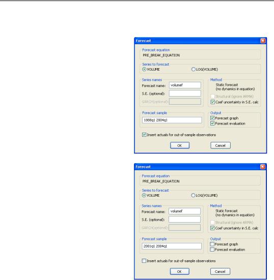
Notice that we have a choice of fore-
casting either volume or
log(volume) . (When you use a function as a dependent variable, EViews offers the choice of forecasting either the function or the underlying variable.) The one we actually care about is volume—taking logs was just a trick to get a better statistical model. Leave the dialog set to forecast volume. Uncheck Forecast graph, Forecast evaluation, and Insert actuals for out-of-sample observations. In the Forecast sample field enter “2001q1 2004q1”. Your dialog should look something like the one shown.
What’s Ahead—21
EViews creates a series of forecast values for volume, storing them in the series VOLUMEF, which now appears in the workfile window. Double-click on  . Choose
View/Graph... in the VOLUMEF window and select Line in the dialog to see the forecast values.
The first thing you’ll notice is that nothing shows up on most of the plot. We asked EViews to start the forecast in January 2001 and that’s what EViews did, so there is no forecast for most of our historical period. Click the  button and enter “2000 @LAST” in the upper field of the Sample dialog. Alternately, use the slider bar to set the sample from 2000q1 to 2004q1. The graph snaps to a close up view of the last few years.
You have a volume forecast. NYSE volume is forecast to rise over the forecast period from
about 750 million shares to nearly 1.2 billion. Mission accomplished.
What’s Ahead
This chapter’s been a quick stroll through EViews, just enough—we hope—to whet your appetite. You can continue walking through the chapters in order, but skipping around is fine too. If you’ll be mostly using EViews files prepared by others, you might proceed to Chapter 3, “Getting the Most from Least Squares,” to dive right into regressions; to

22—Chapter 1. A Quick Walk Through
Chapter 7, “Look At Your Data,” for both simple and advanced techniques for describing your data, or to Chapter 5, “Picture This!,” if it’s graphs and plots you’re after. If you like the more orderly approach, continue on to the next chapter where we’ll start the adventure of setting up your own workfile and entering your own data.
Now it’s time to take a break for real.