

Forecasting—327
0.9eT, 0.81eT, 0.729eT… in the first three forecasting periods. As you can see, the ARMA effect gradually declines to zero.
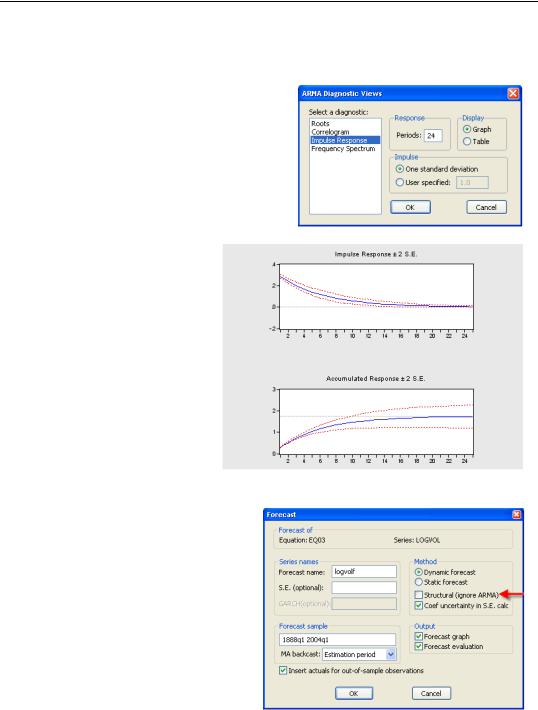
You can see that two elements determine the contribution of ARMA errors to the forecast: the value of the last residual and how quickly the weights decline. The value of the last residual depends on the starting date for the forecast, but the weights can be plotted using ARMA Structure…/Impulse Response.
The weights are multiplied either by the standard error of the regression, if you choose
One standard deviation, or by a value of your own choosing. Here’s the plot for our AR(1) model set to User specified:
1.0. Even after two years, 28 percent of the final residual will remain in the forecast.
Forecasting
When we discussed forecasting in Chapter 8, “Forecasting,” we put off the discussion of forecasting with ARMA errors—because we hadn’t yet discussed ARMA errors. Now we have! The intuition about forecasting with ARMA errors is straightforward. Since errors persist in part from one period to the next, forecasts of the left-hand side variable can be improved by including a forecast of the error term.
EViews makes it very easy to include the contribution of ARMA errors in

328—Chapter 13. Serial Correlation—Friend or Foe?
forecasts. Once you push the  button all you have to do is not do anything—in other words, the default procedure is to include ARMA errors in the forecast. Just don’t check the
Structural (ignore ARMA) checkbox.
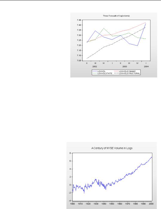
Static Versus Dynamic Forecasting With ARMA errors
When you include ARMA errors in your forecast, you still need to decide between “static” and “dynamic” forecasting. The difference is best illustrated with an example. We have data on NYSE volume through the first quarter of 2004. Let’s forecast volume for the last eight quarters of our sample, based on the model including an AR(1) error. Since we know what actually happened in that period, we can compare our forecast with reality to see how well we’ve done.
Nomenclature hint: This is sometimes called in-sample forecasting, see Chapter 8, “Forecasting.”
The first quarter of our forecast period is 2002q2. First, EViews will multiply the right hand
side variables for 2002q2 by their respective estimated coefficients. Then EViews adds in the contribution of the AR(1) term: 0.8365 times the residual from 2002q1 (the final period
before the forecast began).
The second period of our forecast is 2002q3. Now EViews will multiply the right hand side
variables for 2002q3 by their respective estimated coefficients. Then there’s a choice: should we add in 0.8365 times the residual from 2002q2, or should we use times the
residual from 2002q1? The former is called a static forecast and the latter a dynamic forecast. The static forecast uses all information in our data set, while the dynamic forecast uses only information through the start of the estimation sample. The static forecast uses the best available information, so it’s likely to be more accurate. On the other hand, if we were truly forecasting into an unknown future, dynamic forecasting would be the only option. Static forecasting requires calculation of residuals during the forecast period. If you don’t know the true values of the left-hand side variable, you can’t do that. Therefore dynamic forecasting is generally a better test of how well multi-period forecasts would work when forecasting for real.
ARMA and ARIMA Models—329
Using our AR(1) model, we’ve constructed three forecasts: dynamic, static, and structural (ignore ARMA), this last forecast leaving out the contribution of the ARMA terms entirely. The static and dynamic forecasts are identical for the first period; they’re supposed to be, of course. In general, the static forecast tracks the actual data best, followed by the dynamic forecast, with the structural forecast coming in last.
ARMA and ARIMA Models
The basic approach of regression analysis is to model the dependent variable as a function of the independent variables. The addition of ARMA errors augments the regression model with additional information about the persistence of errors over time. A widely used alterna- tive—variously called Time Series Analysis or Box-Jenkens analysis, or ARMA or ARIMA modeling—directly models the persistence of the dependent variable. Estimation of ARMA or ARIMA models in EViews is very easy. We begin with a short digression into the “unit root problem” and then work through a pure time series model of NYSE volume.
Who Put the I in ARIMA?
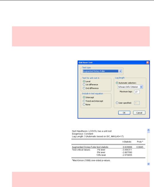
Series that explode over time can be statistically problematic. Most of statistical theory requires that time series be stationary (non-explosive), as opposed to nonstationary
(explosive). This is an oversimplification of some fairly complex issues. But looking at a graph of LOGVOL, it’s clear that volume has exploded over time. This suggests—but doesn’t prove—that a time series model of the level of LOGVOL might be dicey. A
standard solution to this problem is to build a model of the first difference of the variable
330—Chapter 13. Serial Correlation—Friend or Foe?
instead of modeling the level directly. Given such a differenced model, we then need to “integrate” the first differences to recover the levels. So an ARMA model of the first difference is an AR-Integrated-MA, or ARIMA, model of the level.
Hint: If you know dy1 ≡ y1 – y0 , dy2 ≡ y2 – y1 , etc., then you can find y1 by adding dy1 to y0 . You can find y2 by adding dy2 and dy1 to y0 , and so forth. Adding up the first differences is the source of the term “integrated.”
Unit Root Tests
A series that’s stationary in first differences is said to possess a unit root. EViews provides a battery of unit root tests from the View/Unit Root Test… menu. For our purposes, the default test suffices. (The User’s Guide has an extended discussion of both EViews options and of the different tests available.)
For this test, the null hypothesis is that there is a unit root. An excerpt of our test results are shown to the right. Because the hypothesis of a unit root is not rejected, we’ll build a model of first differences.
Hint: The first difference of LOGVOL can be written in two ways: D(LOGVOL) or LOGVOL-LOGVOL(-1). The two are equivalent.
ARMA and ARIMA Models—331
Hint: Once in a great while, it’s necessary to difference the first difference in order to get a stationary time series. If it’s necessary to difference the data d times to achieve stationarity, then the original series is said to be “integrated of order d,” or to be an I(d) series. The complete specification of the order of an ARIMA model is ARIMA(p, d, q), where a plain old ARMA model is the special case ARIMA(p, 0, q).
By the way, the d() function generalizes in EViews so that d(y,d) is the dth difference of Y.
ARIMA Estimation
Here’s a plot of D(LOGVOL). No more exploding.
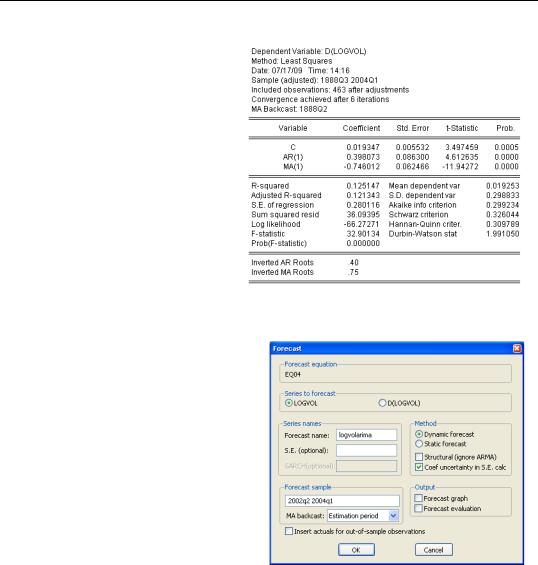
Building an ARIMA model of LOGVOL boils down to building an ARMA model of D(LOGVOL). It’s traditional to treat the dependent variable in an ARMA model as having mean zero. One way to do this is to use the expression “D(LOGVOL)-@MEAN(D(LOGV OL))” as the dependent variable, but it’s just as easy to include a constant in the estimate.
So with that build up, here’s
how to estimate an ARIMA(1,1,1) model in EViews:
ls d(logvol) c ar(1) ma(1)
332—Chapter 13. Serial Correlation—Friend or Foe?
That wasn’t very hard. The results are shown to the right. Both ARMA coefficients are off-the-scale significant. The R2 isn’t very high, but remember that we’re explaining changes—not levels—of volume.
To estimate higher order ARIMA models, just include more AR and MA terms in the command line.
ARIMA Forecasting
Forecasting from an ARIMA model pretty much consists of pushing the  button and then setting the options in the Forecast dialog as you would for any other equation. You’ll notice one new twist: The dependent variable is D(LOGVOL), but EViews defaults to forecasting the level variable, LOGVOL.