

Correcting for Serial Correlation—323
Conveniently, the Breusch-Godfrey test with q lags specified serves as a test against an MA(q) process as well as against an AR(q) process.
Autoregressive Regressive Moving Average (ARMA) Errors
Autoregressive and moving average errors can be combined into an autoregressive-moving average, or ARMA, process. For example, putting an AR(2) together with an MA(1) gives you an ARMA(2,1) process which can be written as ut = r1ut – 1 .
For an ARMA(3,4) model, you would traditionally have to include a separate term for each ARMA lag, such that you would write it in your equation as:
ls y c ar(1) ar(2) ar(3) ma(1) ma(2) ma(3) ma(4)
In EViews, you can just write:
ls y c ar(1 to 3) ma(1 to 4)
It works in the same way for lags; you can write y(-1 to -4) instead of having to write y(-1) y(-2) y(-3) y(-4).
Correcting for Serial Correlation
Now that we know that our stock volume equation has serial correlation, how do we fix the problem? EViews has built-in features to correct for either autoregressive or moving average errors (or both!) of any specified order. (The corrected estimate is a member of the class called Generalized Least Squares, or GLS.) For example, to correct for first-order serial correlation, include “AR(1)” in the regression command just as if it were another variable. The command:
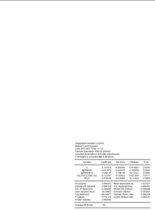
ls logvol c @trend @trend^2 d(log(close(-1))) ar(1)
gives the results shown. The first thing to note is the additional line reported in the middle panel of the output. The serial correlation coefficient, what we’ve called r in writing out the equations, is labeled “AR(1)” and is estimated to equal about 0.84. The associated standard error, t-sta- tistic, and p-value have the usual interpretations. In our equation, there is very strong evidence that the serial correlation coefficient doesn’t equal zero— confirming all our earlier statistical tests.

324—Chapter 13. Serial Correlation—Friend or Foe?
Now let’s look at the top panel, where we see that the number of observations has fallen from 430 to 429. EViews uses observations from before the start of the sample period to estimate AR and MA models. If the current sample is already at the earliest available observation, EViews will adjust the sample used for the equation in order to free up the pre-sample observations it needs.
There’s an important change in the bottom panel too, but it’s a change that isn’t explicitly labeled. The summary statistics at the bottom are now based on the innovations (e) rather than the error (u) . For example, the R2 gives the explained fraction of the variance of the dependent variable, including “credit” for the part explained by the autoregressive term.
Similarly, the Durbin-Watson is now a test for remaining serial correlation after first-order serial correlation has been corrected for.
Serial Correlation and Misspecification
Econometric theory tells us that if the original equation was otherwise well-specified, then correcting for serial correlation should change the standard errors. However, the estimated coefficients shouldn’t change by very much. (Technically, both the original and corrected results are “unbiased.”) In our example, the coefficient on D(LOG(CLOSE(-1))) went from positive and significant to negative and insignificant. This is an informal signal that the dynamics in this equation weren’t well-specified in the original estimate.
Higher-Order Corrections
Correcting for higher-order autoregressive errors and for moving errors is just about as easy as correcting for an AR(1)—once you understand one very clever notational oddity. EViews requires that if you want to estimate a higher order process, you need to include all the lower-order terms in the equation as well. To estimate an AR(2), include AR(1) and AR(2). To estimate an AR(3), include AR(1), AR(2), and AR(3). If you want an MA(1), include MA(1) in the regression specification. And as you might expect, you’ll need MA(1) and MA(2) to estimate a second-order moving average error.
Hint: Unlike nearly all other EViews estimation procedures, MA requires a continuous sample. If your sample includes a break or NA data, EViews will give an error message.
Why not just type “AR(2)” for an AR(2)? Remember that a second-order autoregression has two coefficients, r1 and r2 . If you type “AR(1) AR(2),” both coefficients get estimated. Omitting “AR(1)” forces the estimate of r1 to zero, which is something you might want to do on rare occasion, probably when modeling a seasonal component.
Autoregressive and moving average errors can be combined. For example, to estimate both an AR(2) and an MA(1) use the command:
Correcting for Serial Correlation—325
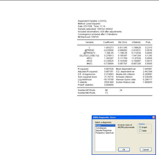
ls logvol c @trend @trend^2 d(log(close(-1))) ar(1) ar(2) ma(1)
The results, shown to the right, give both autoregressive coefficients and the single moving average coefficient. All three ARMA coefficients are significant.
Another Way to Look at the ARMA Coefficients
Equations that include ARMA parameters have an ARMA Structure… view which brings up a dialog offering four diagnostics. We’ll take a look at the Correlogram view here and the Impulse Response view in the next section.
326—Chapter 13. Serial Correlation—Friend or Foe?
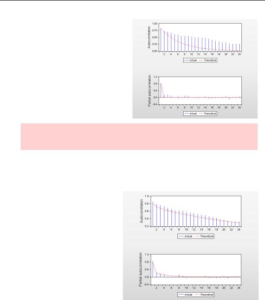
Here’s the correlogram for the volume equation estimated above with an AR(1) specification. The correlogram, shown in the top part of the figure, uses a solid line to draw the theoretical correlogram corresponding to the estimated ARMA parameters. The spikes show the empirical correlogram of the residuals - the same values as we saw in the residual correlogram earlier in the chapter.
Nomenclature Hint: The theoretical correlogram corresponding to the estimated ARMA parameters is sometimes called the Autocorrelation Function or ACF.
The solid line (theoretical) and the top of the spikes (empirical) don’t match up very well, do they? The pattern suggests that an AR(1) isn’t a good enough specification, which we already suspected from other evidence.
Here’s the analogous correlogram from the ARMA(2,1) model we estimated earlier. In this more general model the theoretical correlogram and the empirical correlogram are much closer. The richer specification is probably warranted.
The Impulse Response Function
Including ARMA errors in forecasts sometimes makes big improvements in forecast accuracy a few periods out. The further out you forecast, the less ARMA errors contribute to forecast accuracy. For example, in an AR(1) model, if the autoregressive coefficient is estimated as 0.9 and the last residual is eT , then including the ARMA error in the forecast adds