

Testing for Serial Correlation—319
To plot the autocorrelations of the residuals, click the  button and choose the menu Residual
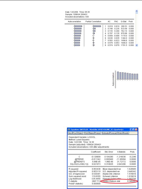
Diagnostics/Correlogram - Q-Sta- tistics.... Choose the number of autocorrelations you want to see—the default, 36, is fine—and EViews pops up with a combined graphical and numeric look at the autocorrelations. The unlabeled
column in the middle of the display, gives the lag number (1, 2, 3, and so on). The column marked AC gives estimated autocorrelations at the corresponding lag. This correlogram shows substantial and persistent autocorrelation.
The left-most column gives the autocorrelations as a bar graph. The graph is a little easier to read if you rotate your head 90 degrees to put the autocorrelations on the vertical axis and the lags on the horizontal, giving a picture something like the one to the right showing slowing declining autocorrelations.
Testing for Serial Correlation
Visual checks provide a great deal of information, but you’ll probably want to follow up with one or more formal statistical tests for serial correlation. EViews provides three test statistics: the Durbin-Watson, the Breusch-Godfrey, and the Ljung-Box Q-statistic.
Durbin-Watson Statistic
The Durbin-Watson, or DW, statistic is the traditional test for serial correlation. For reasons discussed below, the DW is no longer the test statistic preferred by most econometricians. Nonetheless, it is widely used in practice and performs excellently in most situations. The Durbin-Watson tradition is so strong that EViews routinely reports it in the lower panel of regression output.
The Durbin-Watson statistic is unusual in that under the null hypothesis (no serial correlation)

320—Chapter 13. Serial Correlation—Friend or Foe?
the Durbin-Watson centers around 2.0 rather than 0. You can roughly translate between the Durbin-Watson and the serial correlation coefficient using the formulas:
DW = 2 – 2r
r = 1 – (DW ⁄ 2)
If the serial correlation coefficient is zero, the Durbin-Watson is about 2. As the serial correlation coefficient heads toward 1.0, the Durbin-Watson heads toward 0.
To test the hypothesis of no serial correlation, compare the reported Durbin-Watson to a table of critical values. In this example, the Durbin-Watson of 0.349 clearly rejects the absence of serial correlation.
Hint: EViews doesn’t compute p-values for the Durbin-Watson.
The Durbin-Watson has a number of shortcomings, one of which is that the standard tables include intervals for which the test statistic is inconclusive. Econometric Theory and Methods, by Davidson and MacKinnon, says:
…the Durbin-Watson statistic, despite its popularity, is not very satisfactory.… the DW statistic is not valid when the regressors include lagged dependent variables, and it cannot be easily generalized to test for higher-order processes.
While we recommend the more modern Breusch-Godfrey in place of the Durbin-Watson, the truth is that the tests usually agree.
Econometric warning: But never use the Durbin-Watson when there’s a lagged dependent variable on the right-hand side of the equation.
Breusch-Godfrey Statistic
The preferred test statistic for checking for serial correlation is the Breusch-Godfrey. From the  menu choose Residual Diagnostics/Serial Correlation LM Test… to pop open a small dialog where you enter the degree of serial correlation you’re interested in testing. In other words, if you’re interested in firstorder serial correlation change Lags to include to 1.
Testing for Serial Correlation—321
The view to the right shows the results of testing for first-order serial correlation. The top part of the output gives the test results in two versions: an F- statistic and a x2 statistic. (There’s no great reason to prefer one over the other.) Associated p-values are shown next to each statistic. For our stock market volume data, the hypothesis of no serial correlation is easily rejected.
The bottom part of the view provides extra information showing the auxiliary regression used to create the test statistics reported at the top. This extra regression is sometimes interesting, but you don’t need it for conducting the test.
Ljung-Box Q-statistic
A different approach to checking for serial correlation is to plot the correlation of the residual with the residual lagged once, the residual with the residual lagged twice, and so on. As we saw above in The Correlogram, this plot is called the correlogram of the residuals. If there is no serial correlation then correlations should all be zero, except for random fluctuation.
To see the correlogram, choose Residual Diagnostics/Correlogram - Q-statistics… from the  menu. A small dialog pops open allowing you to specify the number of correlations to
show.
The correlogram for the residuals from our volume equation is repeated to the right. The column headed “Q-Stat” gives the LjungBox Q-statistic, which tests for a particular row the hypothesis that all the correlations up to and including that row equal zero. The column marked “Prob” gives the corresponding p-value. Continuing
along with the example, the Q-statistic against the hypothesis that both the first and second correlation equal zero is 553.59. The probability of getting this statistic by chance is zero to three decimal places. So for this equation, the Ljung-Box Q-statistic agrees with the evi-

322—Chapter 13. Serial Correlation—Friend or Foe?
dence in favor of serial correlation that we got from the Durbin-Watson and the BreuschGodfrey.
Hint: The number of correlations used in the Q-statistic does not correspond to the order of serial correlation. If there is first-order serial correlation, then the residual correlations at all lags differ from zero, although the correlation diminishes as the lag increases.
More General Patterns of Serial Correlation
The idea of first-order serial correlation can be extended to allow for more than one lag. The correlogram for first-order serial correlation always follows geometric decay, while higher order serial correlation can produce more complex patterns in the correlogram, which also decay gradually. In contrast, moving average processes, below, produce a correlogram which falls abruptly to zero after a finite number of periods.
Higher-Order Serial Correlation
First-order serial correlation is the simplest pattern by which errors in a regression equation may be correlated over time. This pattern is also called an autoregression of order one, or AR(1), because we can think of the equation for the error terms as being a regression on one lagged value of itself. Analogously, second-order serial correlation, or AR(2), is written
ut = r1ut – 1 + r2ut – 2 + et . More generally, serial correlation of order p, AR(p), is written ut = r1ut – 1 + r2ut – 2 + … + rput – p + et .
When you specify the number of lags for the Breusch-Godfrey test, you’re really specifying the order of the autoregression to be tested.
Moving Average Errors
A different specification of the pattern of serial correlation in the error term is the moving average, or MA, error. For example, a moving average of order one, or MA(1), would be written ut = et + vet – 1 and a moving average of order q, or MA(q), looks like
ut = et + v1et – 1 + … + vqet – q . Note that the moving average error is a weighted average of the current innovation and past innovations, where the autoregressive error is a weighted average of the current innovation and past errors.
Convention Hint: There are two sign conventions for writing out moving average errors. EViews uses the convention that lagged innovations are added to the current innovation. This is the usual convention in regression analysis. Some texts, mostly in time series analysis, use the convention that lagged innovations are subtracted instead. There’s no consequence to the choice of one convention over the other.