


Chapter 13. Serial Correlation—Friend or Foe?
In a first introduction to regression, it’s usually assumed that the error terms in the regression equation are uncorrelated with one another. But when data are ordered— for example, when sequential observations represent Monday, Tuesday, and Wednesday—then we won’t be very surprised if neighboring error terms turn out to be correlated. This phenomenon is called serial correlation. The simplest model of serial correlation, called first-order serial correlation, can be written as:
yt |
= |
bxt + ut |
||||
ut |
= rut – 1 + et, 0 ≤ |
|
r |
|
< 1 |
|
|
|
|||||
|
|
|||||
The error term for observation t, ut , carries over part of the error from the previous period, rut – 1 , and adds in a new innovation, et . By convention, the innovations are themselves uncorrelated over time. The correlation comes through the rut – 1 term. If r = 0.9 , then 90 percent of the error from the previous period persists into the current period. In contrast, if r = 0 , nothing persists and there isn’t any serial correlation.
If left untreated, serial correlation can do two bad things:
•Reported standard errors and t-statistics can be quite far off.
•Under certain circumstances, the estimated regression coefficients can be quite badly biased.
When treated, three good things are possible:
•Standard errors and t-statistics can be fixed.
•The statistical efficiency of least squares can be improved upon.
•Much better forecasting is possible.
We begin this chapter by looking at residuals as a way of spotting visual patterns in the regression errors. Then we’ll look at some formal testing procedures. Having discussed detection of serial correlation, we’ll turn to methods for correcting regressions to account for serial correlation. Lastly, we talk about forecasting.
Fitted Values and Residuals
A regression equation expresses the dependent variable, yt as the sum of a modeled part, bxt , and an error, ut . Once we’ve computed the estimated regression coefficient, bˆ , we can make an analogous split of the dependent variable into the part explained by the regression, and the part that remains unexplained, et ≡ yt – bxt . The explained part, yˆ t , is called the fitted value. The unexplained part, et , is called the residual. The residuals
316—Chapter 13. Serial Correlation—Friend or Foe?
are estimates of the errors, so we look for serial correlation in the errors (ut) by looking for serial correlation in the residuals.
EViews has a variety of features for looking at residuals directly and for checking for serial correlation. Exploration of these features occupies the first half of this chapter. Additionally, you can capture both fitted values and residuals as series that can then be investigated just like any other data. The command fit seriesname stores the fitted values from the most recent estimation and the special series RESID automatically contains the residuals from the most recent estimation.
Hint: Since RESID changes after the estimation of every equation, you may want to use Proc/Make Residual Series… to store residuals in a series which won’t be accidentally overwritten.
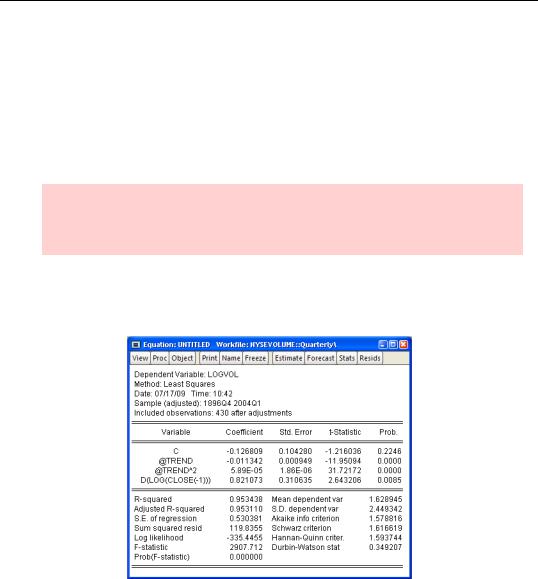
As an example, the first command here runs a regression using data from the workfile “NYSEVOLUME.wf1”:
ls logvol c @trend @trend^2 d(log(close(-1)))
The next commands save the fitted values and the residuals, and then open a group—which we changed to a line graph and then prettied up a little.
fit logvol_fitted
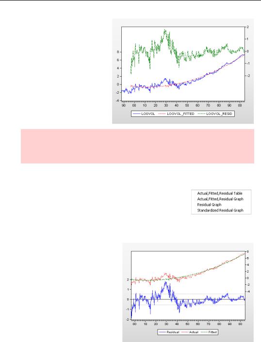
series logvol_resid = logvol - logvol_fitted show logvol logvol_fitted logvol_resid
Visual Checks—317
You’ll note that the model does a good job of explaining volume after 1940, where the residuals fluctuate around zero, and not such a good job before 1940, where the residuals look a lot like the dependent variable.
Econometric hint: We’re treating serial correlation as a statistical issue. Sometimes serial correlation is a hint of misspecification. Although it’s not something we’ll investigate further, that’s probably the case here.
Visual Checks
Every regression estimate comes with views to make looking at residuals easy. If the errors are serially correlated, then a large residual should generally be followed by another large residual; a small residual is likely to be followed by another small residual; and positive followed by positive and negative
by negative. Clicking the  button brings up the Actual, Fitted, Residual menu.
Choosing Actual, Fitted, Residual Graph switches to the view shown to the right. The actual dependent variable (LOGVOL in this case) together with the fitted value appear in the upper part of the graph and are linked to the scale on the righthand axis. The residuals are plotted in the lower area, linked to the axis on the left.
The residual plot includes a solid line at zero to make it easy to visually pick out runs of positive and
318—Chapter 13. Serial Correlation—Friend or Foe?
negative residuals. Lightly dashed lines mark out ±1 standard error bands around zero to give a sense of the scaling of the residuals.
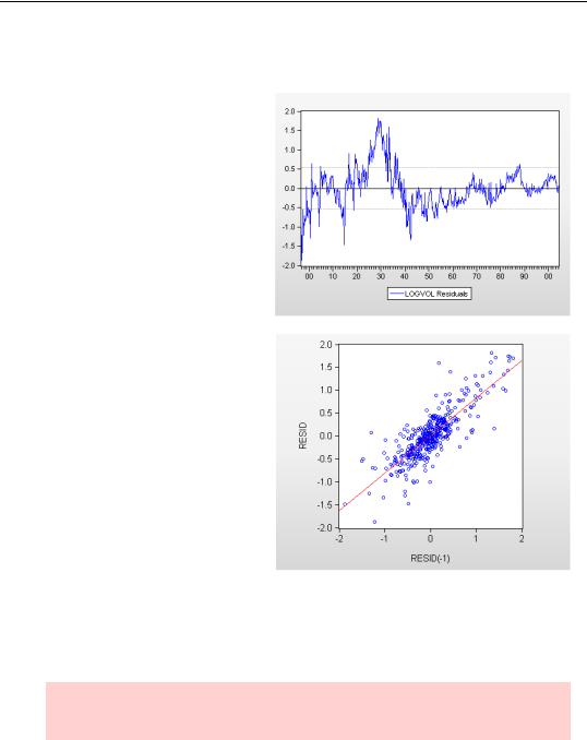
It’s useful to see the actual, fitted, and residual values plotted together, but it’s sometime also useful to concentrate on the residuals alone. Pick
Residual Graph from the Actual, Fitted, Residual menu for this view. In this example there are long runs of positive residuals and long runs of negative residuals, providing strong visual evidence of serial correlation.
Another way to get a visual check is with a scatterplot of residuals against lagged residuals. In the plot to the right we see that the lagged residual is quite a good predictor of the current residual, another very strong indicator of serial correlation.
The Correlogram
Another visual approach to checking for serial correlation is to look directly at the empirical pattern of correlations between residuals and their own past values. We can compute the correlation between et and
et – 1 , the correlation between et and et – 2 , and so on. Since the correlations are of the residual series with its (lagged) self, these are called autocorrelations. If there is no serial correlation, then all the correlations should be approximately zero—although the reported values will differ from zero due to estimation error.
Hint: For the first-order serial correlation model that opens the chapter, ut = rut – 1 + et , the autocorrelations equal r, r2, r3… .