

302—Chapter 12. Everyone Into the Pool
Getting Out of the Pool
Pooled series are plain old series, so the pool object provides a number of tools for manipulating pooled plain old EViews objects in convenient ways. A number of useful procedures involving pools appear under the Proc menu.
Hint: If you don’t see the procedures for pools listed under the Proc menu, be sure that the pool window is active. Clicking the  button in a pool window gets you to the same menu.
Pool Series Generation
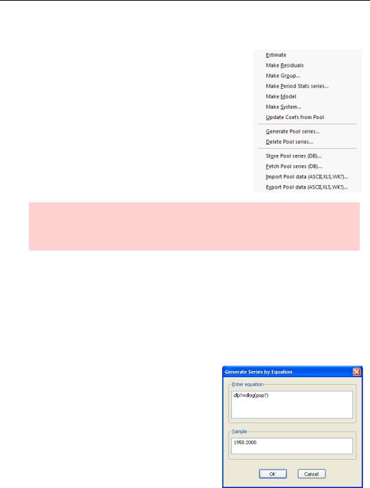
Much of our analysis on the pool has used percentage population growth, measured as D(LOG(POP?)). We might want to generate this as a new series for each country. Manually, we could give six commands of the form:
series dlpcan = d(log(popcan))
series dlpfra = d(log(popfra))
…
To automate the task, hit the  button and enter the equation using a “?” everywhere you want the country identifier to go. The entry “DLP? = D(LOG(POP?))” generates all six series.
Getting Out of the Pool—303
Hint: genr is a synonym for the command series in generating data. Hence the name on the button, “PoolGenr.”
Pool Series Degeneration
To delete a pile of series, choose Delete Pool series…. from the Proc menu. This deletes the series. It doesn’t affect the pool definition in any way.
Making Groups
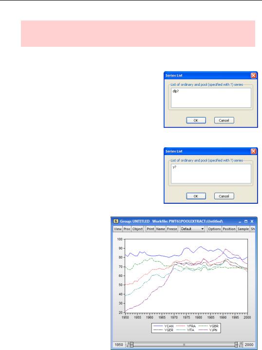
As you’ve seen, there are lots of ways to manipulate a group of pooled series from the pool window. But sometimes it’s easier to include all the series in a standard EViews group and then use group procedures. Plotting pooled series is one such example. Choose Make Group… from the Proc menu and enter the series you want in the Series List dialog. An untitled group will open.
If we like, we could make a quick plot of Y for the pooled series by switching the group to a graph view. (See Chapter 5, “Picture This!”)
304—Chapter 12. Everyone Into the Pool
More Pool Estimation
You won’t be surprised that estimates with pools come with lots of interesting options. We touch on a few of them here. For complete information, see the User’s Guide.
Residuals
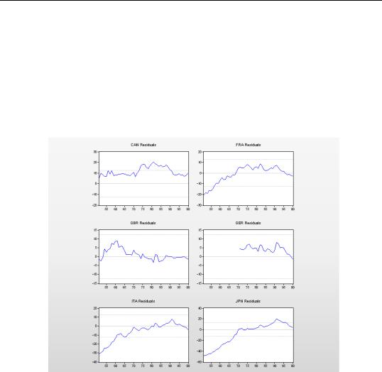
Return to the first pooled estimate in the chapter, the one with a common intercept for all series. Pick the menu View/Residuals/Graphs. The first thing you’ll notice is that squeezing six graphs into one window makes for some pretty tiny graphs.
Residuals are supposed to be centered on zero. The second thing you’ll notice is that the residuals for Canada are all strongly positive, those for Germany are mostly positive and Italy’s residuals are nearly all negative, so the residuals are not centered on zero. That’s a hint that the country equations should have different intercepts.
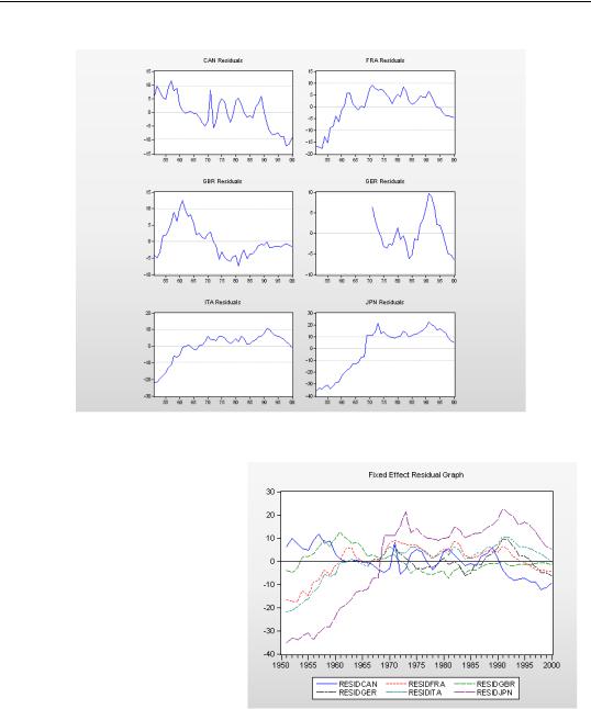
We can get different intercepts by specifying fixed effects. Let’s look at the residual plots from the fixed effects equation we estimated. This time, each country’s residual is centered around zero.
More Pool Estimation—305
Grabbing the Residual Series
If six graphs in one window is looking a little hard to read, think what sixty-six graphs would look like! Proc/Make Residuals generates series for the residuals from each country, RESIDCAN, RESIDFRA, etc., and puts them into a group window. From there, it’s easy to make any kind of group plot we’d like. Here’s one to which we’ve added a title and zero line. It’s pretty clear from this picture that the fit for Japan is problematic.
Our model doesn’t take into account the post-War Japanese recovery - and it shows! (If this were a real research project we’d have to stop and deal with the misspecification issue. Employing the literary device suspension of disbelief, we’ll just proceed onward.)
306—Chapter 12. Everyone Into the Pool
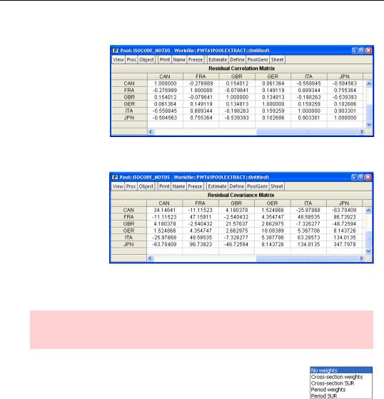
Residual Correlations
Clicking on
View/Residuals/Correlation Matrix gives us a table showing the correlation of the residuals. The correlations involving Japan
and Italy are particularly high.
The menu
View/Residuals/Covariance Matrix gives variances and covariances instead of correlations. Note that the variance of the residuals
for Japan, 347.8, is ten times the variance for Canada.
Generalized Least Squares and Heteroskedasticity Correction
Relaxation hint: This is a book about EViews, not an econometrics tome. If the title of this section just pushed past your comfort zone, skip ahead to the next topic.
One of the assumptions underlying ordinary least squares estimation is that all observations have the same error variance and that errors are uncorrelated with one another. When this assumption isn’t true reported standard errors from ordinary least squares tend to be off and you forego information that can lead to improved estimation efficiency.
The tables above suggest that our pooled sample has both problems: correlation across observations and differing variances. EViews offers a number of options in the Weights menu in the Pool Estimation dialog, shown to the right, for dealing with heteroskedasticity. We’ll touch on a couple of them.
More Pool Estimation—307
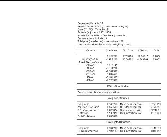
Country Specific Weights
To allow for a different variance for each country, choose Crosssection weights. Compare these estimates to those we saw in
Everyone Into the Pool May Not Be Fun, on page 294. The estimated effect of growth is much smaller. The standard error is also smaller, but it shrunk by less than the coefficient did. It would have been nicer if the t-statistic had become larger rather than smaller, at least if “nicer” is interpreted as providing support to our preconceived notions.
As you might guess, the menu choice Period weights is analogous to Cross-section weights, allowing for different variances for each time period instead of each country.
308—Chapter 12. Everyone Into the Pool
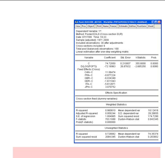
Cross-country Correlations
To account for correlation of errors across countries as well as different variances, choose Crosssection SUR. This option requires balanced samples —ones that all have the same start and end dates. So if your pool isn’t balanced— ours isn’t—you’ll also need to check the Balance Sample checkbox at the lower right of the dialog. The estimated effect of population growth is now quite small, but statistically very significant.
Nomenclature hint: SUR stands for Seemingly Unrelated Regression.
Period SUR provides the analogous model where errors are correlated across periods within each country’s observations.
More Options to Mention
If you’re in an exploring mood, note that EViews will do random effects as well as fixed effects (in the Estimation method field of the Specification tab of the Pool Estimation dialog) and Period specific coefficients just as it does Cross-section specific coefficients
(Regressors and AR() terms). The Options tab provides a variety of methods for robust estimation of standard errors, and also options for controlling exactly how the estimation is done. These are, of course, discussed at length in the User’s Guide.