

Playing in the Pool—Data—297
Playing in the Pool—Data
Pooled series are just plain-old series that share a naming convention. All the usual operations on series work as expected. But there are some extra features so that you can examine or manipulate all the series in a pool in one operation.
Hint: It’s fine to have multiple pool objects in the workfile. They’re just different lists of identifiers, after all.
Spreadsheet Views
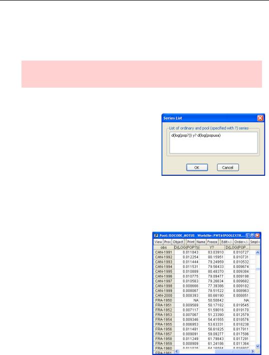
Pools have two special spreadsheet views, stacked and unstacked, chosen by pushing the  button or choosing the View/Spreadsheet (stacked data)… menu. For either view, the first step is to specify the desired series when the Series List dialog opens. Enter the names of the series you’d like to see, using the conventions that a series with a question mark means replace that question mark with each of the country ids
in turn. A series with no a question mark means use the series as usual, repeated for each country. The way we’ve filled in the dialog here asks EViews to display D(LOG(POPCAN)), D(LOG(POPFRA)), etc., for YCAN, YFRA, etc., and for D(LOG(POPUSA)) separately.
Stacked View
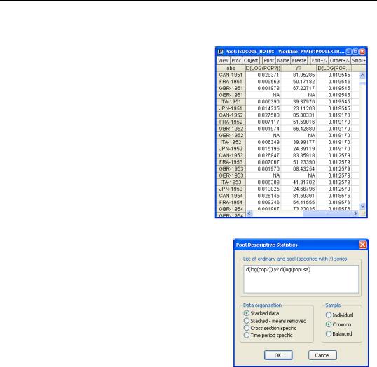
The spreadsheet opens with all the data for Canada followed by all the data for France, etc. The data for POPUSA gets repeated next to each country. Notice how the identifier  in the obs column gives the crosssection identifier followed by the date—in other words, country and year.
This is called the stacked view. You can imagine putting together all the data for Canada, then stacking on all the data for France, etc. We’ll return to the idea of a stacked view when we talk about loading in pooled data below.
298—Chapter 12. Everyone Into the Pool
Unstacked View
Re-arranging the spreadsheet into the “usual order,” that is by date, is called the unstacked view. Clicking the  button flicks back- and-forth between stacked and unstacked views.
Pooled Statistics
The Descriptive Statistics… view offers a number of ways to slice and dice the data in the pool. We’ve put two pooled series (with the “?” marks) and one non-pooled series in the dialog so you can see what happens as we try out each option.
First, look at the Sample radio buttons on the right. The presence of missing data, NAs, means that the samples available for one series may differ from the sample available for another. You can see above, for example, that Canada, France, and Great Britain have data starting in 1950, but that German data begins later. Common sample instructs EViews to
use only those observations available for all countries for a particular series, while Balanced sample requires observations for all countries for all series entered in the dialog. Individual sample means to use all the observations available.
Playing in the Pool—Data—299
Stacked Data Statistics
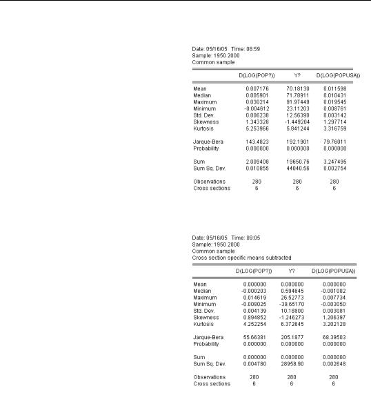
The default Data Organization is
Stacked data, which stacks the series for all countries together for the purpose of producing descriptive statistics. For example, we see that GDP per capita in our six pooled countries averaged just over 70 percent of U.S. GDP per capita. (Y is measured relative to U.S. GDP.)
Stacked - Means Removed
Specifying Stacked - means removed in Descriptive Statistics produces some pretty funny looking output, but it turns out that this method is just what we want for answering certain questions. EViews subtracts the means for each country before generating the descriptive statistics. As a consequence, the means are always zero, which looks pretty funny.
The raison d’être for Stacked - means removed is to see statistics other than the means and medians. (The medians aren’t zero, but they’re pretty close.)
According to the Stacked data statistics,
the standard deviation of annual U.S. population growth was 3/10ths of one percent, while the standard deviation for the pooled countries was 6/10ths of one percent. This looks like population growth was much more variable for the countries in the pooled sample. Whether this is the correct conclusion depends on a subtle point. Some of the countries have relatively high population growth and some have lower growth. The standard deviation for Stacked data includes the effect of variability across countries and across time, while the standard deviation reported for the United States is looking only at variability across time. The Stacked - means removed report takes out cross-country variability, reporting the time
300—Chapter 12. Everyone Into the Pool
series variation within a country, averaged across the pooled sample. This standard deviation is just over 4/10ths of one percent. So the typical country in our pooled sample has only slightly higher variability in population growth than the United States.
The choice to remove means or not before computing descriptive statistics isn’t a right-or- wrong issue. It’s a way of answering different questions.
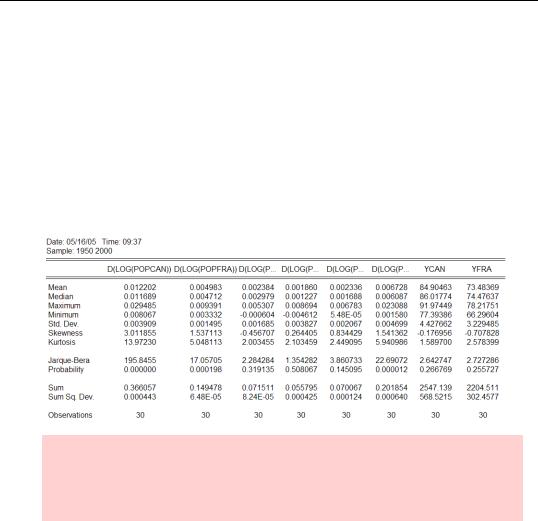
Cross Section Specific Statistics
Choosing the Cross section specific radio button generates descriptive statistics for each country separately, one column for each country for each series. In our example we have six reports from D(LOG(POP?)), six from Y?, and one from D(LOG(POPUSA)), an excerpt of which is shown below.
Empirical aside: If you’re following along on the computer, you can scroll the output to see that three of the countries in the pooled sample have population growth standard deviations much lower than the U.S. and three have standard deviations a little above that of the U.S.
Playing in the Pool—Data—301
Time Period Specific Statistics
Time period specific is the flip side of Cross section specific. Time period specific pools the whole sample together and then computes mean, median, etc., for each date.
You can save the time period
specific statistics into series. Click the  button and choose Make Periods Stats series….
Check boxes for the desired descriptive statistics and EViews will (1) create the requested series, YMEAN, YMED, etc., and (2) open an untitled group displaying the new series.