

Chapter 12. Everyone Into the Pool
Suppose we want to know the effect of population growth on output. We might take Canadian output and regress it on Canadian population growth. Or we might take output in Grand Fenwick and regress it on Fenwickian population growth. Better yet, we can pool the data for Canada and Grand Fenwick in one combined regression. More data—better estimates. Of course, we’ll want to check that the relationship between output and population growth is the same in the two countries before we accept combined results.
Pooling data in this way is so useful that EViews has a special facility—the “pool” object— to make it easy to work with pooled data. We begin this chapter with an illustration of using EViews’ pools. Then we’ll look at some slightly fancy arrangements for handling pooled data.
Getting Your Feet Wet
The file “PWT61PoolExtract.wf1” (available from the EViews website) contains annual data on population and output (relative to the United States) extracted from the Penn World Tables for the G7 countries (Canada, France, Germany, Great Britain, Italy, Japan, and the United States). The first thing you’ll notice is that there are lots of population and output series, one for each country. We use pools to study behavior common to all the countries. The second thing you’ll notice is that series names have two parts: a series component identifying the series, and a cross-section component identifying the crosssection element—the country in this example. So POPCAN is population for Canada and POPFRA is population for France. YCAN is Canadian output and YFRA is French output. There’s just one rule you have to remember about series set up in a pool:
•Pooled series aren’t any different from any other series; they’re simply ordinary series conveniently named with common components.
In other words, pool series have neither any special features nor any special restrictions. The only thing going on is that their names are set up conveniently to identify the country (or other cross-sectional element) with which they’re associated. For example, the command:
292—Chapter 12. Everyone Into the Pool
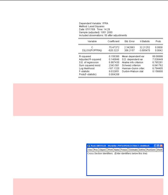
ls yfra c d(log(popfra))
gives us the regression of output on population growth for France. The reported effect of population growth is statistically significant and rather large. (Given historical magnitudes in French rates of population growth, the effect accounts for a decrease in output of about 10 percent relative to US output.)
Reverse causation alert: There’s good reason to believe that countries becoming richer leads to lower population growth. Thus there’s a real issue of whether we’re picking up the effect of output on population growth rather than population growth on output. The issue is real, but it hasn’t got anything to do with illustrating the use of pools, so we won’t worry about it further.
Into the Pool
•Pooled series aren’t any different from any other series, but Pool objects let us do some nifty tricks with them.
The first step in pooled analysis is to give EViews a list of the suffixes, CAN, FRA, etc., that identify the countries. Click on the  button, select New Object...
and choose Pool.
Hint: The cross-section identifier needn’t be placed as a suffix. You can stick it anywhere in the series name so long as you’re consistent.
Getting Your Feet Wet—293
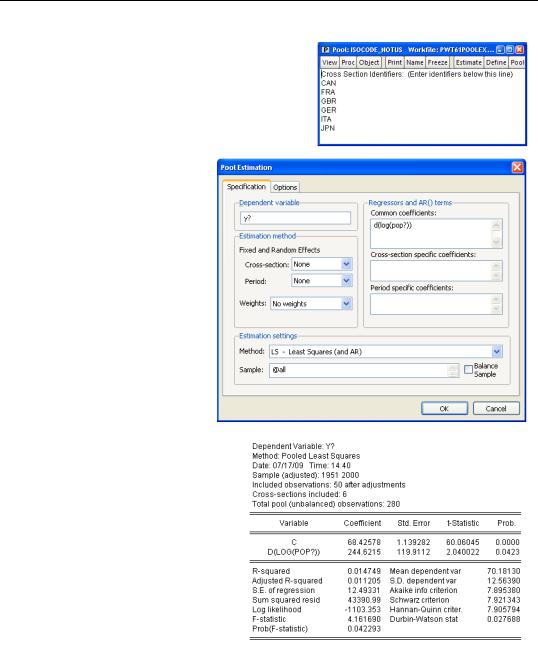
Simply type the country identifiers—one per line—into the blank area and then name the pool by clicking on the  button. In our example the window ends up looking as shown to the right.
Click on the  button in the Pool window. For this first example, enter “Y?” in the Dependent variable field and “C D(LOG(POP?))” in the
Common coefficients field.
•In a pooled analysis, the “?” in the variable names gets replaced with the ids listed in the pool object.
Clicking  gives us a regression that’s just like the regression on French data reported above— except that this time we’ve combined the data for all six countries. Let’s see what’s changed. First, we have 280 observations instead of 50. Second, the reported effect of population has switched sign. The French-only result was negative as theory predicts. The pooled result is positive.
294—Chapter 12. Everyone Into the Pool
Everyone Into the Pool May Not Be Fun
The advantage of pooling data is that a great deal of data is brought to bear on the problem. The potential disadvantage is that a simple pool forces the coefficients to be identical across countries. Does this make sense in our example? We probably do want the coefficient on population growth to be the same for each country, because the theory isn’t of much use if population growth doesn’t have a predictable effect. In contrast, there’s no reason for the intercept to be the same for each country. We
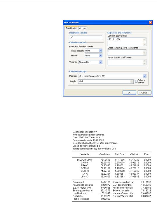
know that countries have different levels of GDP for reasons unrelated to population growth. Let’s retry this estimate with an individual intercept for each country. Go back to the estimation dialog and move the constant from the Common coefficients field into
Cross-section specific coefficients.
Now we’re asking for a separate intercept for each country. The estimated effect of population growth is negative as we had expected. And the increased sample size has raised the t-statistic on population growth from 3 to 5.
Getting Your Feet Wet—295
Observation about life as a statistician: Running estimates until you get results that accord with prior beliefs is not exactly sound practice. The risk isn’t that the other guy is going to do this intentionally to fool you. The risk is that it’s awfully easy to fool yourself unintentionally.
There’s nothing special about moving the constant term into the Cross-section specific coefficients field. You can do the same for any variable you think appropriate.
Fixed Effects
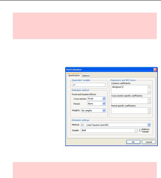
Okay—that first sentence was a fib. There is something special about the constant. The cross-section specific constant picks up all the things that make one country different from another that aren’t included in our model. Such differences occur so frequently that EViews has a built-in facility for allowing for such country-specific constants. Country-specific constants are called fixed effects. Push  again, take the constant term out of the specification entirely and set Estimation method to Crosssection: Fixed.
Hint: The econometric issues surrounding fixed effects in pools are the same as for panels. See Chapter 11, “Panel—What’s My Line?”
296—Chapter 12. Everyone Into the Pool
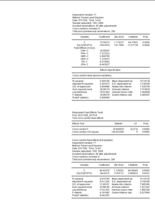
Fixed effect estimation puts in an intercept for every country, and changes slightly how the results are reported. The intercept is now reported in two parts. (Nothing else in the report changes.) The line marked “C” reports the average value of the intercept for all the countries in the sample. The lines marked for the individual countries give the country’s intercept as a deviation from that overall average. In this example the overall average intercept is 76 and the intercept for Canada is 96 (20 above 76).
Testing Fixed Effects
Fixed effects specifications are common enough that EViews builds in a test for country specific intercepts against a single, common, intercept. After a pooled estimate specifying fixed effects, choose  and then the menu
Fixed/Random Effects Testing/Redundant Fixed Effects - Likelihood Ratio. Both F- and x2- tests appear at the top of the view. Since the hypothesis of a common intercept is wildly rejected, there’s more to the fixed effect specification than just that it gives results that we like.