

Estimating your first regression in EViews—13
Looking at a spreadsheet of a group with two series leaves us in the same situation we were in earlier with a spreadsheet view of a single series: too many numbers. A good way to look for a relationship between two series is the scatter diagram. Click on the  button and choose
Graph.... Then select Scatter as the Graph Type on the left-hand side of the dialog that pops up. To add a regression line, select Regression line from the Fit lines dropdown menu. The default options for a regression line are fine, so hit
 to dismiss the dialog.
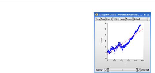
We can see that the straight line gives a good rough description of how log volume moves over
time, even though the line doesn’t hit very many points exactly.
The equation for the plotted line can be written algebraically as y = aˆ + bˆ t . aˆ is the intercept estimated by the computer and bˆ is the estimated slope. Just looking at the plot, we can see that the intercept is roughly -2.5. When LOGVOL looks to be about 4. Reaching back—possibly to junior high school—for the formula for the slope gives us an approximation for bˆ .
ˆ ≈ 4 – (–2.5) = 0.01625
------------------------
b 400 – 0
An eyeball approximation is that LOGVOL rises sixteen thousandths—a bit over a percent and a half—each quarter.
Estimating your first regression in EViews
The line on the scatter diagram is called a regression line. Obviously the computer knew the parameters aˆ when it drew the line, so backing the parameters out by eye may bring back fond memories, but otherwise is unnecessarily convoluted. Instead, we turn now to regression analysis, the most important tool of econometrics.
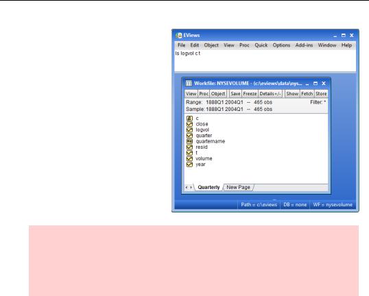
You can “run a regression” either by using a menu and dialog or by typing a command. Let’s try both, starting with the menu and dialog method. Pick the menu item Quick/Estimate Equation… at the top of the EViews window. Then in the upper field type “logvol c t”.
Alternatively, type in the EViews command pane:
ls logvol c t
as shown below.
14—Chapter 1. A Quick Walk Through
In EViews you specify a regression with the ls command followed by a list of variables. (“LS” is the name for the EViews command to estimate an ordinary Least Squares regression.) The first variable is the dependent variable, the variable we’d like to explain—LOGVOL in this case. The rest of the list gives the independent variables, which are used to predict the dependent variable.
Hint: Sometimes the dependent variable is called the “left-hand side” variable and the independent variables are called the “right-hand side” variables. The terminology reflects the convention that the dependent variable is written to the left of the equal
sign and the independent variables appear to the right, as, for example, in log(volumet) = a + bt .
Whoa a minute. “LOGVOL” is the variable we created with the logarithm of volume, and “T” is the variable we created with a time trend. But where does the “C” in the command come from? “C” is a special keyword signaling EViews to estimate an intercept. The coefficient on the “variable” C is aˆ , just as the coefficient on the variable T is bˆ .
Estimating your first regression in EViews—15
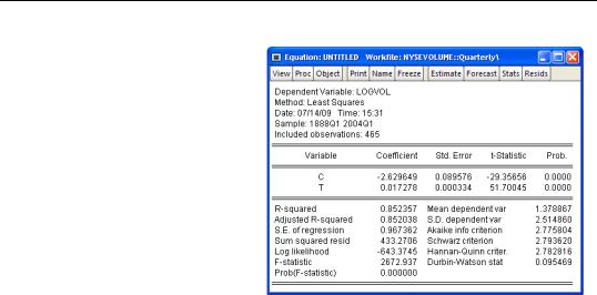
Whether you use the menu or type a command, EViews pops up with regression results.
EViews has estimated the intercept aˆ = –2.629649 and the slope bˆ = 0.017278 . Note that
our eyeballing wasn’t far off!
We’ve estimated an equation explaining LOGVOL that reads:
LOGVOL = – 2.629649 + 0.017278t
Having seen the picture of the scatter diagram on page 13, we know this line does a decent job of summarizing log(volume) over more than a century. On the other hand, it’s not true that in each and every quarter LOGVOL equals – 2.629649 + 0.017278t , which is
what the equation suggests. In some quarters volume was higher and in some the volume was lower. In regression analysis the amount by which the right-hand side of the equation misses the dependent variable is called the residual. Calling the residual e (“e” stands for “error”) we can write an equation that really is valid in each and every quarter:
LOGVOL = – 2.629649 + 0.017278t + e
Since the residual is the part of the equation that’s left over after we’ve explained as much as possible with the right-hand side variables, one approach to getting a better fitting equation is to look for patterns in the residuals. EViews provides several handy tools for this task which we’ll talk about later in the book. Let’s do something really easy to start the exploration.
16—Chapter 1. A Quick Walk Through
Just as there are multiple ways to view series and groups, equations also come with a variety of built in views. In the equation window choose the  button and pick
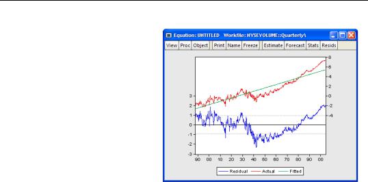
Actual, Fitted, Residual/Actual, Fitted, Residual Graph. The view shifts from numbers to a picture.
There are lots of details on this chart. Notice the two different vertical axes, marked on both the left and right sides of the graph, and the three different series that appear. The horizontal axis shows the date. The actual values
of the left-hand side variable—called “Actual”—and the values predicted by the right-hand
side—called “Fitted”—appear in the upper part of the graph. In other words, the thick upper “line” marked “Actual” is log(volume) and the straight line marked “Fitted” is
– 2.629649 + 0.017278t .
Actual and Fitted are plotted along the vertical axis marked on the right side of the graph; fitted values rising roughly from -2 to 8. Residual, plotted in the lower portion of the graph, uses the legend on the left hand vertical axis.
Whether we look at the top or bottom we see that the fitted line goes smack though the middle of log(volume) in the early part of the sample, but then the fitted value is above the
actual data from about 1930 through 1980 and then too low again in the last years of the sample. If we could get an equation with some upward curvature perhaps we could do a better job of matching up with the data. One way to specify a curve is with a quadratic equation such as:
log(volumet) = a + b1t + b2t2 + e
For this equation we need a squared time trend. As in most computer programs, EViews uses the caret, “^”, for exponentiation. In the command pane type:
series tsqr = t^2
Estimating your first regression in EViews—17
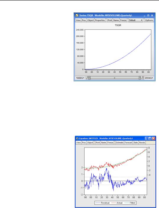
To see that this does give us a bit of a curve, double-click  . Then in the series window choose
View/Graph... and select Line to see a plot showing a reassuring upward curve.
Close the equation window and any series windows that are cluttering the screen. (Don’t close the workfile window.)
Now let’s estimate a regression including t2 to see if we can do a better job of matching the data. EViews is generally quite happy to let you use a mathematical expres-
sion right in the LS command, rather than having to first generate a variable under a new name. To illustrate this capability type in the command pane:
ls log(volume) c t tsqr
We’ve typed in “log(volume)” instead of the series name LOGVOL, and could have typed “t^2” instead of tsqr: thus illustrating that you can use either a series name or an algebraic expression in a regression command.
EViews provides estimates for all three coefficients, aˆ , bˆ 1 , and bˆ 2 .
Has adding t2 to the equation given a better fit? Let’s take a look at the residuals for this new equation. Click View/Actual, Fitted, Residual/Actual, Fitted, Residual Graph again. The fitted line now does a much nicer job of matching the long
run characteristics of
log(volume). In particular, the residuals over the last several decades are now flat rather than trending strongly upward. This new equation is noticeably better at fitting recent data.