


Chapter 11. Panel—What’s My Line?
Time series data typically provide one observation in each time period; annual observations of GDP for the United States would be a classic example. In the same way, cross section data provide one observation for each place or person. We might, for example, have data on 2004 GDP for the United States, Canada, Grand Fenwick, etc. Panel data combines two dimensions, such as both time and place; for example, 30 years of GDP data on the United States and on Canada and on Grand Fenwick.
Broadly speaking, we want to talk about three things in this chapter. First, we’ll talk about why panel data are so nifty. Next comes a discussion of how to organize panel data in EViews. Finally, we’ll look at a few of EViews’ special statistical procedures for panel data.
What’s So Nifty About Panel Data?
Panel data presents two big advantages over ordinary time series or cross section data. The obvious advantage is that panel data frequently has lots and lots of observations. The not always obvious advantage is that in certain circumstances panel data allows you to control for unobservables that would otherwise mess up your regression estimation.
Panels can be big
It’s helpful to think of the observations in a time series as being numbered from 1 to T, even though EViews typically uses dates like “2004q4” rather than 1, 2, 3… as identifiers. Cross section data are numbered from 1 to N, it being something of a convention to use T for time series and N for cross sections. Using i to subscript the cross section and t to subscript the time period, we can write the equation for a regression line as:
yit = a + bxit + uit
With a panel, we are able to estimate the regression line using N × T observations, which can be a whole lot of data, leading to highly precise estimates of the regression line. For example, the Penn World Table (Alan Heston, Robert Summers and Bettina Aten, Penn World Table Version 6.1, Center for International Comparisons at the University of Pennsylvania (CICUP), October 2002) has data on 208 countries for 51 years, for a total of more than 10,000 observations. We’ll use data from the Penn World Table for our first examples.
Using panels to control for unobservables
A key assumption in most applications of least squares regression is that there aren’t any omitted variables which are correlated with the included explanatory variables. (Omitted variables cause least squares estimates to be biased.) The usual problem is that if you don’t observe a variable, you don’t have much choice but to omit it from the regression. When

276—Chapter 11. Panel—What’s My Line?
the unobserved variable varies across one dimension of the panel but not across the other, we can use a trick called fixed effects to make up for the omitted variable. As an example, suppose y depends on both x and z and that z is unobserved but constant for a given country. The regression equation can be written as:
yit = a + bxit + [gzi + uit]
where the variable z is stuffed inside the square brackets as a reminder that, just like the error term u, z is unobservable.
Hint: The subscript on z is just i, not it, as a reminder that z varies across countries but not time.
The trick of fixed effects is to think of there being a unique constant for each country. If we call this constant ai and use the definition ai = a + gzi , we can re-write the equation with the unobservable z replaced by a separate intercept for each country:
yit = ai + bxit + uit
EViews calls ai a cross section fixed effect.
The advantage of including the fixed effect is that by eliminating the unobservable from the equation we can now safely use least squares. The presence of multiple observations for each country makes estimation of the fixed effect possible.
We could have just as easily told the story above for a variable that was constant over time while varying across countries. This would lead to a period fixed effect. EViews panel features allow for cross section fixed effects, period fixed effects, or both.
Setting Up Panel Data
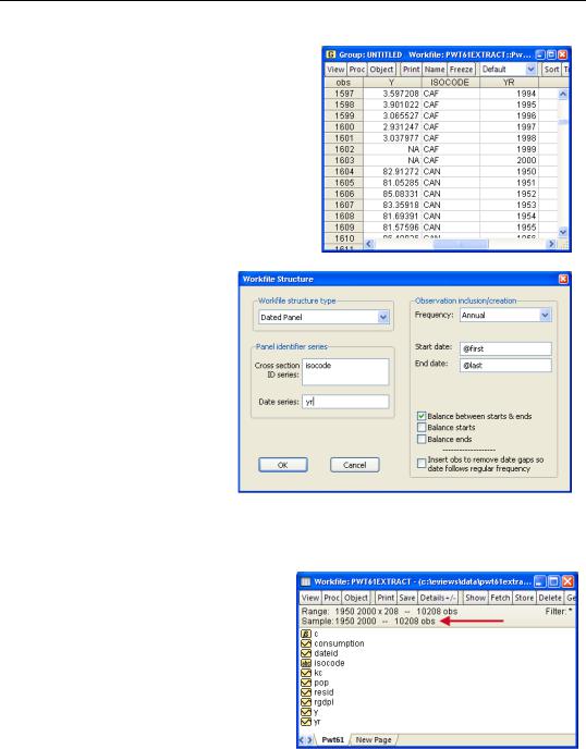
The easiest way to set up a panel workfile is to start with a nonpanel workfile in which one series identifies the period and one series identifies the cross section. The file “PWT61Extract.wf1” has information on both real GDP relative to the United States and on population for a large number of countries for half a century. It also contains a series, ISOCODE, that holds an abbreviation for each country and a series, YR, for the year.
Hint: If two dimensions can be used rather than one, why not three dimensions rather than two? Why not four dimensions? EViews only provides built-in statistical support for two-dimensional panels. In the section Fixed Effects With and Without the Social Contrivance of Panel Structure, below, you’ll learn a technique for handling fixed effects without creating a panel structure. The same technique can be used for estimating fixed effects in third and higher dimensions.
Setting Up Panel Data—277
The figure to the right shows observations 1597 through 1610, which happen to be the last few observations for the Central African Republic and the first few observations for
Canada. To us humans, it’s clear that these are observations for i = CAF,CAN and for t = 1994…2000 and then starting over with t = 1950… . In order to set up a
panel structure, we need to share this kind of understanding with EViews.
Structuring a panel workfile
To change from a regular to a panel structure, use the
Workfile structure dialog. Double click on Range in the upper pane of the workfile window, or use the menu
Proc/Structure/Resize Current Page. Choose Dated Panel for the Workfile structure type and then specify the series containing the cross section (i) and date (t) identifiers. EViews re-organizes the workfile to have a panel
structure (the re-organized workfile is available in the EViews web site as “PWT61PanelExtract.wf1”).
EViews announces the panel aspect of the workfile structure by changing the Range field in the top panel of the workfile window. We now have 208 cross sections for data from 1950 through 2000.
278—Chapter 11. Panel—What’s My Line?
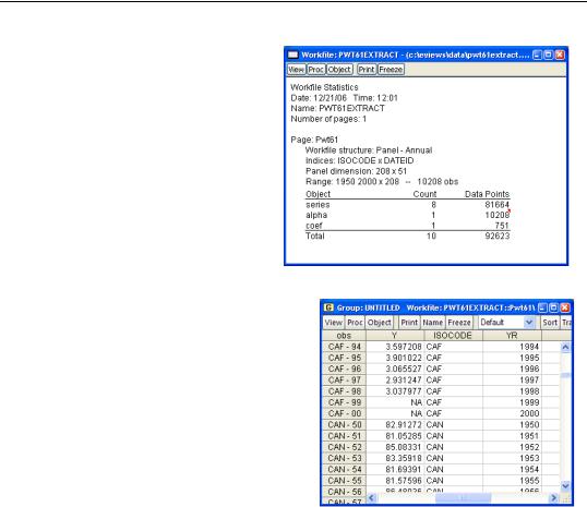
More information about the structure of the workfile is available by pushing the  button and choosing Statistics from the menu.
Let’s take another look at our data, this time as displayed in the panel workfile. Now the obs column correctly identifies each data point with both country code and year.
That’s about all you need to know to set up a panel workfile. One more option is worth mentioning. Should you “balance?”
A panel is said to be balanced when every cross section is observed for the same time period. The Penn World Table data are balanced, since there are observations for 1950 through 2000 for every country—although
quite a few observations are simply marked NA (not available). If you look at the workfile, you’ll see that all the data for the Central African Republic is missing until 1960. (The Central African Republic became independent on August 13, 1960.) The creators of the Penn World Table might have simply omitted these years for the Central African Republic, giving us an unbalanced panel. EViews default (if you leave the check box Balance between starts & ends in the Workfile structure dialog checked) is to make a balanced workfile by inserting empty rows of data where needed. Use Balance between starts & ends unless you have a reason not to do so. (See the User’s Guide for further discussion.)
Panel Estimation
Not that it was much trouble, but we didn’t restructure the workfile just to get a prettier display for spreadsheet views. Let’s work through an estimation example.
Panel Estimation—279
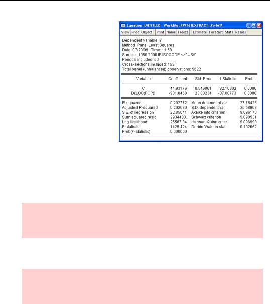
There’s a general notion from classical Solow growth theory that high population growth leads to lower per capita output, conditional on available technologies. We can test this theory by regressing gross domestic product per capita relative to the United States on the rate of population growth, measured as the change in the log of population. Results from a simple regression seem to support such a theory. At least, we can say that the coefficient is statistically significant. In fact, looking at the p-
value, the coefficient is off-the-scale significant.
But is the effect of population growth important? We can try to get a better handle on this by comparing a couple of countries; let’s use the Central African Republic and Canada, since they’re at opposite ends of the development spectrum. Set the sample using:
smpl if isocode=”CAF” or ISOCODE=”CAN”
Reminder: Variable names aren’t case sensitive in EViews (“isocode” and “ISOCODE” mean the same thing), but string comparisons using “=” are. In this particular data set country identifiers have been coded in all caps. “CAN” works. “can” doesn’t.
Now open a window on population growth with the command:
show d(log(pop))
Hint in two parts: The function d() takes the first difference of a series, and the first difference of a log is approximately the percentage change. Hence “d(log(pop))” gives the percentage growth of population.

280—Chapter 11. Panel—What’s My Line?
Hint: Lags in panel workfiles work correctly—in other words, EViews knows that a lag means the previous observation for the same country. Notice in the window to the right that the 1950 value of D(LOG(POP)) is—correctly— NA. Even though the observation for the year 2000 for Canada appears immediately before 1950 Switzerland in the spreadsheet, EViews understands that the observations are not sequential.
Use the  button to choose
Descriptive Statistics & Tests/Stats by Classification…. Use ISOCODE as the classifying variable.
The average value of population growth was 2.2 percent per year in the Central African Republic and 1.6 percent in Canada. If we multiply the difference in population growth rates, 0.008, by the estimated regression coefficient, -901, we predict that relative GDP in the Central African Republic should be 7 percentage points lower than in Canada. Population growth appears to have a very large effect.
Convenience hint: It wasn’t necessary to restrict the sample to the two countries of interest. Limiting the sample just made the output window shorter and easier to look at.
Panel Estimation—281
Is the apparent effect of population growth on output real, or is it a spurious result? It’s easy to imagine that population growth is picking up the effect of omitted variables that we can’t measure. To the extent that the omitted variables are constant for each country, fixed effects estimation will control for the omissions.
Econometric digression: The regression output includes a hint that something funky is going on. The Durbin-Watson statistic (see Chapter 13, “Serial Correlation—Friend or Foe?”) indicates very, very high serial correlation. This suggests that if the error for a country in one year is positive then it’s positive in all years, and if it’s negative once then it’s always negative. High serial correlation in this context provides a hint that we’ve left out country specific information.
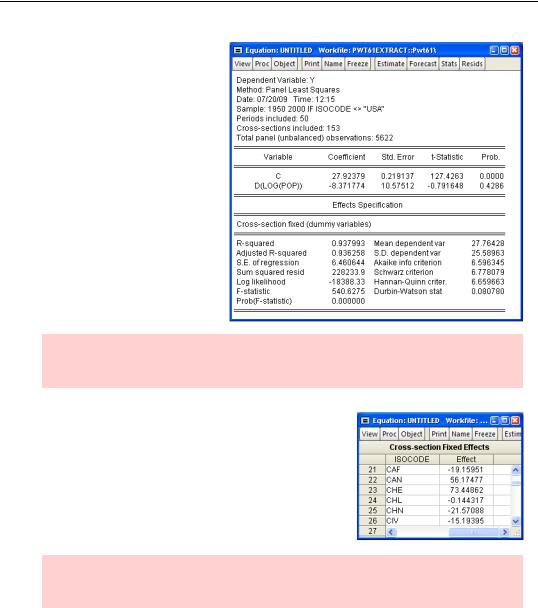
Setting the sample back to everything except the United States, click the  button and then choose the
  tab. Set Effects specification to Cross-sec- tion Fixed. This instructs EViews to include a separate intercept, ai , for each country.
282—Chapter 11. Panel—What’s My Line?
In our new regression results, the effect of population growth is reduced to about one 1/100th of the previous estimate. This confirms our suspicion that the previous estimate had omitted variables—and apparently ones that mattered a lot.
Hint: Fixed/Random Effects Testing offers a formal test for the presence of fixed effects. Look for it on the View menu.
We can take a look at the estimated values of the fixed effects for each country by looking at the Fixed/Random Effects/Cross-section Effects view. The reported values of the cross-section fixed effects are the intercept for country i, ai, less the average intercept. So it’s not very surprising that the effect for Canada is positive and the effect for the Central African Republic is negative.
Hint: When using fixed effects, the constant term reported in regression output is the average value of ai .