


Have A Match?—255
Have A Match?
One key to thinking about which data should be collected in a single EViews page is that all the series in a page share a common identifier. One page might hold quarterly series, where the identifier is the date. Another page might hold information about U.S. states, where the identifier might be the state name or just the numbers 1 through 50. What you can’t have is one page where some series are identified by date and others are identified by state.
Reminder: The identifier is the information that appears on the left in a spreadsheet view.
So far, the examples in this chapter have all used dates for identifiers. Because EViews has a deep “understanding” of the calendar, it knows how to make frequency conversions; for example, translating monthly data to quarterly data. So, while data of different frequencies needs to be held in different pages, linking between pages is straightforward.
What do you do when your data series don’t all have an identifier in common? EViews provides a two-step procedure:
•Bring all the data which does share a common identifier into a page, creating as many different pages as there are identifiers.
•Use “match-merge” to connect data across pages.
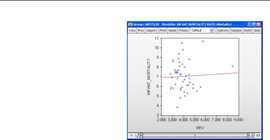
The workfile “Infant Mortality Rate.wf1” holds two pages with data by state. The page Mortality contains infant mortality rates and the page Revenue contains per capita revenue. Is there a connection between the two? Excerpts of the data look like:
There are days when computers are incredibly annoying. The connection between pages is obvious to us, but not to the computer, because the observations aren’t quite parallel in the two pages. The infant mortality data includes an observation for the District of Columbia;
256—Chapter 9. Page After Page After Page
the revenue data doesn’t. The identifier for the former is a list of observation numbers 1 through 51. For the latter, the identifier is observation numbers 1 through 50. Starting with Florida, there’s no identifier in common between the two series because Florida is observation 10 in one page and observation 9 in the other page. Just matching observations by identifier won’t work here. Something more sophisticated is needed.
Matching through Links
You can think of the match process as what computer scientists call a “table look-up.” Each time we need a value for REV, we want EViews to go to the Revenue page and look up the value with the same state name in the Mortality page.
We understand that “state” is the meaningful link between the data in the two different pages. We’ll tell EViews to bring the data from the Revenue page into the Mortality page by creating a link, and then filling in the Properties of the link with the information needed to make a match.
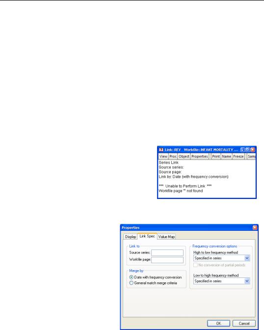
Click on the Mortality tab to activate the Mortality page. Then create a new link named REV using the menu Object/New Object/Series Link. The object  appears in the workfile window with a pink background to indicate a link and a question mark showing that the link hasn’t been specified. Double-clicking
  opens a view with an error message indicating that the properties of the link haven’t been specified yet.
Click the  button and then the Link Spec tab. The default dialog asks about frequency conversions, which isn’t what we need. Click the General match merge criteria radio button in the Merge by field.
Have A Match?—257
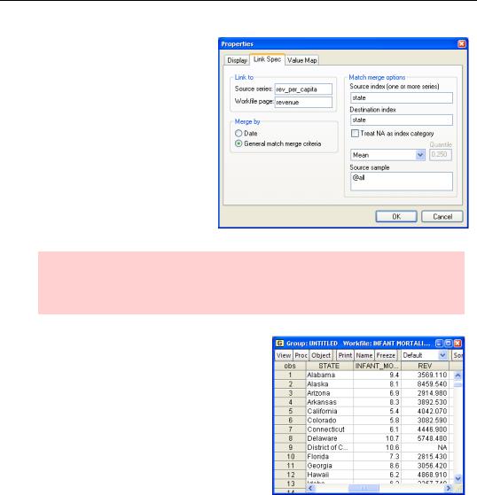
Notice that we now have a new set of fields on the right side of the dialog. Fill out the dialog with the
Source series and Workfile page in the Link to field. Since we want to match observations that have the same state names, enter STATE in both the Source index and Destination index fields. When you close the dialog you’ll see that the link icon has switched to  , indicating that the link is now complete.
Hint: You may find it more intuitive to think of the Link to field as the “Link from” field. Remember that you’re specifying the data source here. The destination is always the active page.
A quick glance at the data shows that EViews has made the correct, obvious (to us) connection.
258—Chapter 9. Page After Page After Page
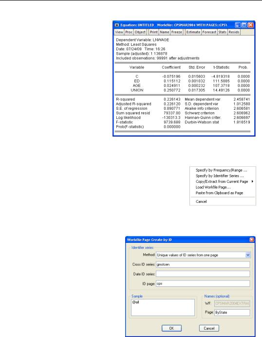
We can now use REV just like any other series. EViews will bring data in from the Revenue page each time it’s needed. For example, a scatter diagram of infant mortality against per capita revenue shows a slight, and surprising, positive association. (The positive association is attributable to the one outlier. Drop Alaska and the picture shifts to a slight negative relation.)
In this example we’ve used links to match in a case where there really was a common identifier, the computer just didn’t know it. Next we
turn to matching up series with fundamentally different identifiers.
Matching When The Identifiers Are Really Different
In this next example, our main data set holds observations on individuals. We’re going to hook up these individual observations with data specific to each person’s state of residence. In order to show off more EViews features, we’ll generate the state-by-state data by taking averages from the individual level data.
For a real problem to work on, we’re going to try to answer whether higher unionization rates raise wages for everyone, or whether it’s just for union members. We begin with a collection of data, “CPSMar2004Extract.wf1”, taken from the March 2004 Current Population Survey. We have data for about 100,000 individuals on wage rates (measured in logs, LNWAGE), education (ED), age (AGE), and whether or not the individual is a union member (UNION, 1 if union member, 0 if not). The identifier of this data set is the observation number for a particular individual.
Our goal is to regress log wage on education, age, union membership, and the fraction of the population that’s unionized in the state. The difficulty is that the unionized fraction of the state’s population is naturally identified by state. We need to find a mechanism to match individual-identified data with the state-identified data. We’ll do this in several steps.
Matching When The Identifiers Are Really Different—259
Let’s first make sure that unionization matters at least for the person in the union. The regression results here show a very strong union effect. Controlling for education and age, being a union member raises your wage by about 25 percent!
Specifying A Page By Identifier Series
Our next step is to create a page holding data aggregated to the state level. We want our new page to contain one observation for each of the states observed in the individual data. Clicking on the New Page tab brings up a menu including the choice Specify by Identifier Series…, which (not surprisingly) is just what we need to specify an identifier series for a new page. In our original page the state identifier is in the
series GMSTCEN, so that’s what we’ll use as the identifier for the new page.
Choosing Specify by Identifier Series… brings up the Workfile Page Create by ID dialog. Enter GMSTCEN in the Cross ID series: field. It’s optional, but we’ve also entered a name for the new page in the Page field at the lower right.
260—Chapter 9. Page After Page After Page
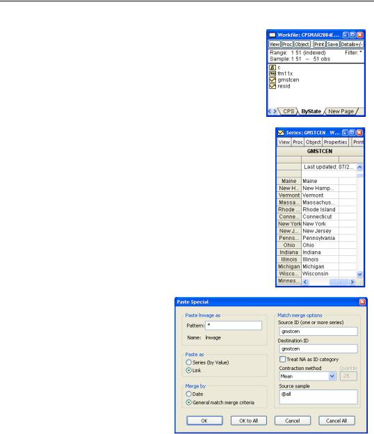
The new page opens containing just the series GMSTCEN. Okay, the new page also contains FM11X—but that’s only because FM11X is a value map holding the names of each state.
If we double-click on GMSTCEN, we see that GMSTCEN has also supplied the identifier series for this page, which appears in the left-most, shaded, column of the spreadsheet. Now that we have a page identified by state, we need to fill it up with state-by-state data. One easy method is copy-and-paste. Go back to the individual data page (Cps). Ctrl-click on LNWAGE, ED, AGE, and UNION to select the relevant series. Copy, and then click back on the ByState tab.
Choose Paste from the context menu. Because Paste and Paste Special are the same here, this brings up the Paste Special dialog. We’ll discuss the Match merge options further in a bit, but EViews has done it’s usual good job of guessing what we want done. For now, just note that the field Contraction method is set to Mean and hit the  button.
Matching When The Identifiers Are Really Different—261
EViews has pasted data into the ByState page using what’s called a “match-merge.” In this case, we’ve gotten the obvious and desired result. The ED series in the ByState page gives the average number of years of education in each state; the UNION series gives the percent unionized, etc. Let’s back up and talk separately about the “match” step and the “merge” step.
Fib Warning: In fact, we haven’t gotten the desired result for a subtle reason involving the sample. Finding the error lets us explore some more features in the next section, Contracted Data. For the moment, we’ll pretend everything is okay.
Ex-post obvious hint: When you average a 0/1 variable like UNION, you get the fraction coded as a “1.” That’s because adding up 0/1 observations is the same as counting the number of 1’s. So taking the average counts the number of 1’s and then divides by the number of observations.
The match step connects the identifiers across pages. In this case, we want to connect observations for individuals and observations for states according to whether they have the same state (GMSTCEN) value.
The merge step maps the large number of observations for individuals into a single value for each state in the ByState page. The default contraction method, Mean, is to average the values for individuals within a state.