


Renaming, Deleting, and Saving Pages—243
If all you want to do is copy the contents of the existing page into a new page, simply dragging the page tab and dropping it on the New Page tab of any workfile. A plus (“+”) sign will appear when your cursor is over an appropriate area.
Messing up hint: EViews doesn’t have an Undo function. When you’re about to make a bunch of changes to your data and you’d like to leave yourself a way to back out, consider using Copy/Extract from Current Page to make a copy of the active page. Then make the trial changes on the copy. If things don’t work out, you still have the original data unharmed on the source page.
Renaming, Deleting, and Saving Pages
To rename, delete, or save a page, right-click on the page tab to bring up a context menu with choices to let you—no surprises here—rename, delete, or save the page. The only mild subtlety is that saving a page actually saves an entire workfile containing that page as its only contents. You can also save a page as a workfile on the disk by using the Proc/Save Current Page… menu.
Hint: Save Workfile Page… will write Excel files, text files, etc., as well as EViews workfiles.
Backwards compatibility hint: The page feature was first introduced in EViews 5. There are three options if you want a friend with an earlier version to be able to read the data:
•Tell them to upgrade to the current release. There are lots of nifty new features.
•Early versions of EViews will read the first page of a multi-page workfile just fine, but ignore all other pages. So if the workfile has only a single page or if the page of interest is the first one created (the left-most page on the row of page tabs), then there’s no problem. If not, you can reorder the pages by dragging the page tabs and dropping them in the desired position. Keep in mind that when reading a file, earlier versions ignore object types that hadn’t yet been invented when the earlier version was released.
•Use Save Workfile Page… to save the page of interest in a standalone workfile.
244—Chapter 9. Page After Page After Page
Multi-Page Workfiles—The Most Basic Motivation
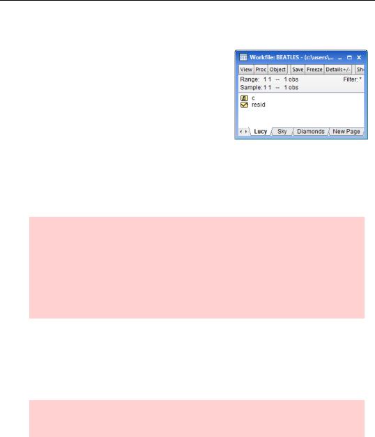
We’ll get to some fancy uses of pages shortly. But don’t overlook the simplest reason for using multipage workfiles: If you have sets of data that you want to keep in one collection, just make each one a page in a workfile. As in the example appearing to the right, it’s perfectly okay if the sets of data are unrelated.
To use a particular page, click on the appropriate tab at the bottom of the workfile window, and you’re in business.
Multiple Frequencies—Multiple Pages
In Chapter 2, “EViews—Meet Data,” we wrote
Hint: Every variable in an EViews workfile shares a common identifier series. You can’t have one variable that’s measured in January, February, and March and a different variable that’s measured in the chocolate mixing bowl, the vanilla mixing bowl, and the mocha mixing bowl.
Subhint: Well, yes actually, you can. EViews has quite sophisticated capabilities for handling both mixed frequency data and panel data. These are covered later in the book.
It is now “later in the book.”
All the data in a page within a workfile share a common identifier. For example, one page might hold quarterly data and another might hold annual data. So if you want to keep both quarterly and annual data in one workfile, set up two pages. Even better, you can easily copy data from one page to another, converting frequencies as needed.
Hint: EViews will convert between frequencies automatically, or you can specify your preferred conversion method. More on this below.
The workfile “US Output.wf1” (available on the EViews website) holds data on the U.S. Index of Industrial Production (IP) and on real Gross Domestic Product (RGDP). In contrast to GDP numbers, which are computed quarterly, industrial production numbers are available monthly. For this reason, industrial production is the output measure of choice for comparison with monthly series such as unemployment or inflation. Since the industrial
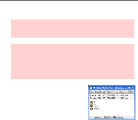
Multiple Frequencies—Multiple Pages—245
production numbers are available more often and sooner, they’re also used to predict GDP. Our task is to use industrial production to forecast GDP.
Hint: http://research.stlouisfed.org/fred2/ is an excellent source for U.S. macroeconomic data. Among other virtues, FRED can make you an Excel file that EViews will read in about two seconds flat.
’nother hint: You can use EViews to search and read data directly from FRED. Select
File/Open/Database... from the main EViews menu and select FRED database. EViews will open a window for examining the FRED database – click on the Easy Query button to search the database for series using names, descriptions, or other characteristics. Once you find the desired series, highlight the series names and rightmouse click or drag-and-drop to send the data into a new or existing workfile. See the User’s Guide for more detail.
Initially, our workfile has two pages. Indpro has monthly industrial production data and Gdpc96 has quarterly GDP data.
To analyze the relation between RGDP and IP, we have to get them into the same page for two reasons:
•Mechanically, only one page is active at a time, so everything we want to use jointly had better be on that page.
•To relate one series to another, at least if we
want to use a regression, observations have to match up. This implies that all the series in a regression need to have the same identifier and therefore the same frequency.
EViews provides a whole toolkit of ways to move series between pages and to convert frequencies, which we’ll take a look at now.
246—Chapter 9. Page After Page After Page
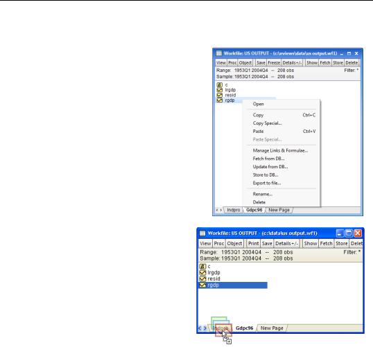
Copy-and-Paste and Drag-and-Drop
Let’s decide to work at a monthly frequency. One approach is to click on the Gdpc96 page tab to make it the active page, then select RGDP and use the right-click context menu to
Copy.
Next, click to activate on the Indpro page and paste.
Equivalently, you can copy RGDP by drag- and-drop the RGDP icon onto the Indpro tab. The icon will display a small plus sign when it is ready to be dropped.
Multiple Frequencies—Multiple Pages—247
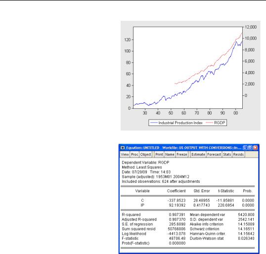
However you copy the data, RGDP appears in the Indpro page (not shown). A dual-scale graph gives a quick look at how the two series relate.
SIP and RGDP are measured in completely different units. IP is simply an index set to 100 in 1997. RGDP is annualized and measured in billions of 1996 dollars. To find a conversion formula, we regress the latter on the former. So when the industrial production number is announced each month, we can get a sneak preview of real GDP with the conversion:
RGDP = – 338 + 92 × IP .
Up-Frequency Conversions
Hold on one second. If GDP is only measured quarterly, how did we manage to use GDP data in a monthly regression? After all, monthly GDP data doesn’t exist!
If you were hoping the good data fairy waived her monthly data wand—and will do the same for you—well, sorry that’s not what happened. Instead, EViews applied a low-to-high frequency data conversion rule. In this case, EViews used a default rule. Let’s go over what rules are available, discuss how you can make your own choice rather than accept the default, and then look at how the defaults get set.
248—Chapter 9. Page After Page After Page
Hint: Low-to-high frequency conversion means from annual-to-quarterly, quarterly-to- monthly, annual-to-daily, etc.
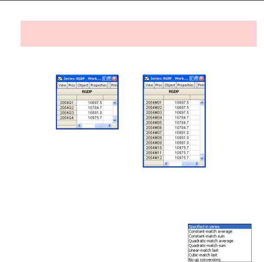
As background, let’s take a look at quarterly GDP values for the year 2004 and the monthly values manufactured by EViews.
We can see that EViews copied the value of GDP in a given quarter into each month of that quarter. That’s a reasonable thing to do. If all we know was that GDP in the first quarter was running at a rate of a trillion dollars a year, then saying that GDP was running at a trillion a year in January, a trillion a year in February, and a trillion a year in March seems like a good start.
What else could we have done? The full set of options is shown at the right. The first choice, Specified in series, isn’t an actual conversion method: It signals to use whichever method is set as the default in the series being copied.
Constant-match average
In the case we’re looking at, the conversion method applied
(by default) was Constant-match average. This instruction parses into two parts: “constant” and “match average.” “Constant” means uses the same number in each month in a quarter. “Match average” instructs EViews that the average monthly value chosen has to match the quarterly value for the corresponding quarter.
At this point you may be muttering under your breath, “What do these guys mean, ‘the average monthly value?’ There only is one monthly value.” You have a good point! When converting from low-to-high frequency, saying “constant - match average” is just a convoluted way of saying “copy the value.” As we’ve seen, that’s exactly what happened above.

Multiple Frequencies—Multiple Pages—249
Later, we’ll see conversion situations where constant-match average is much more complex.
Constant-match sum
Suppose that instead of GDP measured at an annual rate, our low frequency variable happened to be total quarterly sales. In a conversion to monthly sales, we’d like the converted January, February, and March to add up to the total of first quarter sales. Constant-match sum takes the low frequency number and divides it equally among the high frequency observations. If first quarter sales were 600 widgets, Constant-match sum would set January, February, and March sales to 200 widgets each.
Quadratic-match sum and Quadratic-match average
In 2004, GDP rose every quarter. It’s a little strange to assume that GDP is constant across months within a quarter and then jumps at quarter’s end. Quadratic conversion estimates a smooth, quadratic, curve using the data from the current quarter and the previous and succeeding quarters. This curve is then used to interpolate the data within the quarter. “Match average” forces the average of the interpolated numbers to match the original quarterly figure, while “match sum” matches on the sum of the generated high frequency numbers.
Linear-match last and Cubic-match last
Both Linear-match last and Cubic-match last begin by copying the quarterly (more generally, the low frequency source value) into the last monthly observation in the corresponding quarter (more generally, the last corresponding high frequency date). Values for the remaining months are set by linear interpolation between final-months-in-the-quarter for Linearmatch last and by interpolating along natural cubic splines (see the User’s Guide for a definition) for Cubic-match last.
Down-Frequency Conversions
There’s something slightly unsatisfying about low-to-high frequency conversion, in that we’re necessarily faking the data a little. There isn’t any monthly GDP data. All we’re doing is taking a reasonable guess. In contrast, high-to-low frequency conversion doesn’t involve making up data at all.
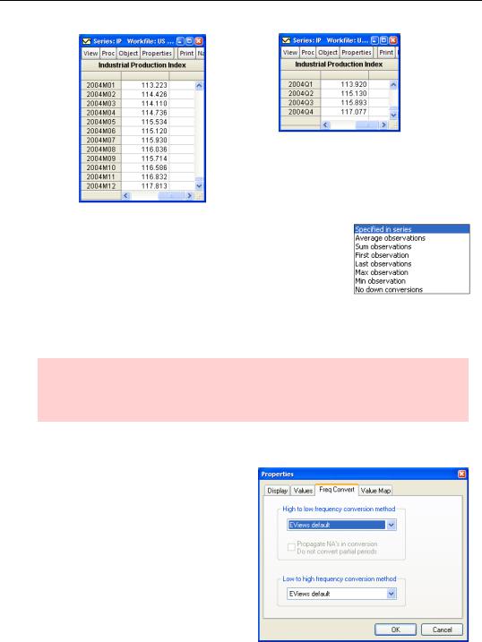
If we copy IP from the monthly Indpro page and paste it into the quarterly Gdpc96 page we see the following:
250—Chapter 9. Page After Page After Page
EViews has applied the default high-to-low frequency conversion procedure, which is to average the monthly observations within each quarter. The meanings of the high-to-low frequency conversion options are pretty straightforward. Sum observations adds up the monthly observations within a quarter. If we had sales for January, February, and March we would use a Sum observations conversion to get total first quarter sales.
First, Last, Max, and Min Observation all pick out one month within the quarter and use the value for the quarterly value.
Hint: First observation and Last observation are especially useful in the analysis of financial price data, where point-in-time data are often preferred over time aggregated data.
Default Frequency Conversions
Every series has built-in default frequency conversions, one for high-to-low and one for low-to-high. These defaults are used when you copy-and-paste from one page or workfile to another. To change the default choices, open the series and click the  button. Choose the Freq Convert tab to access available choices.
The overall EViews default is changed using the menu Options/General
Options/Series and Alphas/Frequency Conversion….