


8—Chapter 1. A Quick Walk Through
Hint: The new sample applies to all our work until we change it again, not just this one graph. Note the change in the Sample: line of the workfile window.
Generating a new series
Let’s turn to another approach to thinking about trading volume. Our first line graph (before we shortened the sample) presented a picture which looks a lot like exponential growth over time. A standard trick for dealing with exponential growth is to look at the logarithm of a variable, relying on the identity y = egt logy = gt . In order to look at the trend in the log instead of in the level, we’ll create a new variable named LOGVOL which equals the log of VOLUME. This can be done either with a dialog or by typing a command. We’ll do the former first. Choose the menu item Quick/Generate Series… to bring up
a dialog box. In the upper field, type “logvol=log(volume)”. Notice that in the lower field the sample is still set to use only the 21st century part of our data. This matters, as we’ll see in a moment.
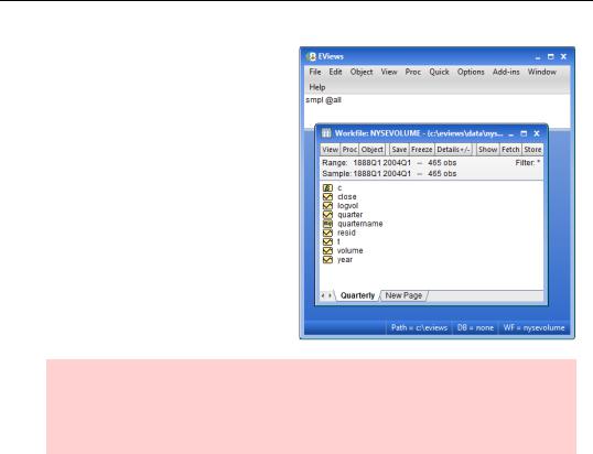
The workfile window now has a new object,  .
.

Generating a new series—9
Double-click  and then scroll the window so that the beginning of 2000 is at the top. You’ll see a window looking something like the one shown here.
Starting in 2001 we see numbers. Before 2001, only the letters “NA”. There are two lessons here:
•EViews operates only on data in the current sample.
When we created LOGVOL the sample began in 2001. No values were generated for earlier dates.
•EViews marks data that are not available with the symbol NA.
Since we didn’t generate any values for the early
years for LOGVOL, there aren’t any values available. Hence the NA symbols.
Since we’re trying to look at all the available data, we want to change the sample to include, well the whole sample. One way to do this is to use the menu selection Quick/Sample….
Another way to change the sample is to double-click on the sample line in the upper pane of the workfile window—right where the arrow’s pointing in the picture on the right.
To illustrate another alternative, we’ll type our first command.
The workfile window and the series window appear in the lower section of the master EViews window. The upper area is reserved for typing commands, and, not surprisingly, is called
the command pane. The command smpl is used to set the sample; the keyword @all signals EViews to use all available data in the current sample. Type the command:
smpl @all
in the command pane and end with the Enter key.
Hint: Almost everything in EViews can be done either by typing commands or by choosing a menu item. The choice is a matter of personal preference.
10—Chapter 1. A Quick Walk Through
You can see that the sample in the workfile window has changed back to 1888Q1 through 2004Q1.
Historical hint: Ever wonder why so many computer commands are limited to four letters? Back in the early days of computing, several widely used computers stored characters “four bytes to the word.” It was convenient to manipulate data a “word” at a time. Hence the four letter limit and commands spelled like “smpl”.
Now that you’ve set the sample to include all the data, let’s generate LOGVOL again, this time from the command line. Type:
series logvol = log(volume)
in the command pane and hit Enter. (This is the last time I’ll nag you about hitting the Enter key. I promise.)
Looking at a pair of series together—11
Again double-click on LOGVOL to check that we now have all our data. Then use the View menu to choose View/Graph... and select Line graph. The line graph for LOGVOL—the logarithm of our original VOLUME variable— appears. What we see is not quite a straight line, but it’s a lot closer to a straight line—and a lot easier to look at—than our graph of the original VOLUME variable.
Hint: Menu items, both in the menu bar at the top of the screen and menus chosen from the button bar, change to reflect the contents of the currently active window. If the menu items differ from those you expect to see, the odds are that you aren’t looking at the active window. Click on the desired window to be sure it’s the active window.
We might conclude from looking at our LOGVOL line graph that NYSE volume rises at a more or less constant percentage growth rate in the long run, with a lot of short-run fluctuation. Or perhaps the picture is better represented by slow growth in the early years, a drop in volume during the Great Depression (starting around 1929), and faster growth in the postWar era. We’ll leave the substantive question as a possibility for future thought and turn now to building a regression model and making a forecast of future trading volume.
Looking at a pair of series together
Our line graph goes quite far in giving us a qualitative understanding of the behavior of volume over time. For a quantitative understanding, we’d like to put some numbers to the upward trending picture of LOGVOL. If we have a variable t representing time (0, 1, 2, 3…), then we can represent the idea of an upward trend with the algebraic model:
log(volumet) = a + bt
where the coefficient b gives the quarterly increase in LOGVOL.

12—Chapter 1. A Quick Walk Through
To get started we need to create the variable t. In the command pane at the top of the EViews screen type:
series t = @trend
“@TREND” is one of the many functions built into EViews for manipulating data. Double-click on  and you’ll see something like the screen shown.
Since we want to think about how volume behaves over time, we want to look at the variables T and LOGVOL together. In EViews a collection of series dealt with together is called a Group. To create a group including T and LOGVOL, first click on  . Now, while holding down the Ctrl-key, click on
  . Then right-click highlighting Open, bringing up the context menu as shown and choose as Group.
The group shows time and log volume, that is, the series T and LOGVOL, together. Just as there are multiple ways to view a series, there are also a number of group views. Here’s the spreadsheet view.