

232—Chapter 8. Forecasting
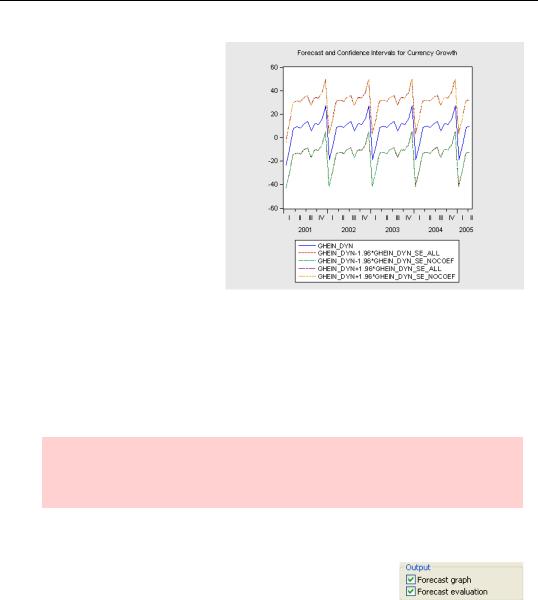
We’ve stored the standard error for our dynamic forecast including coefficient uncertainty as GHEIN_DYN_SE_ALL and analogously, without coefficient uncertainty, under GHEIN_DYN_SE_NOCOEF. Here’s a plot of the forecast value and confidence bands, measured as the forecast minus 1.96 standard errors through the forecast plus 1.96 standard errors. You can see that the difference between the confidence intervals with and without coefficient uncertainty is all but invisible to the eye. That’s one
reason people often don’t bother including coefficient uncertainty.
For the record, here’s the command that produced the plot (before we added the title and tidied it up):
plot ghein_dyn ghein_dyn-1.96*ghein_dyn_se_all ghein_dyn- 1.96*ghein_dyn_se_nocoef ghein_dyn+1.96*ghein_dyn_se_all ghein_dyn+1.96*ghein_dyn_se_nocoef
Hint: This plot shows two forecasts and two associated sets of confidence intervals. Usually, you want to see a single forecast and its confidence intervals. EViews can do that graph automatically, as we’ll see next.
Forecast Evaluation
EViews provides two built-in tools to help with forecast evaluation: the Output field checkboxes Forecast graph and Forecast evaluation.
Forecast Evaluation—233
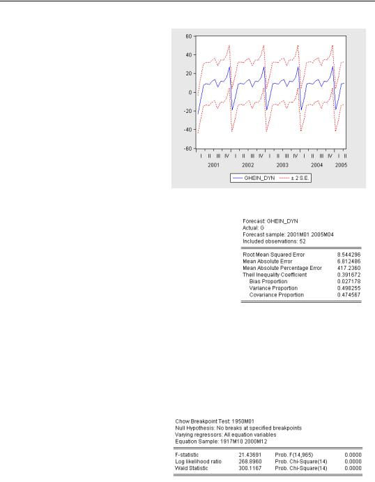
The Forecast graph option automates the 95% confidence interval plot.
The Forecast evaluation option generates a small table with a variety of statistics for comparing forecast and actual values. The Root Mean Squared Error (or RMSE) is the standard deviation of the forecast errors. (See the User’s Guide for explanations of the other statistics.)
Our forecasts aren’t bad, but the confidence intervals shown in the graph above are fairly wide given the observed movement of G. Similarly, the RMSE is not
small compared to the standard deviation of G. Looking back at our plot of out-of-sample forecasts versus actuals, one is struck with the fact that the forecasts take wider swings than the data. In the data plot that opened the chapter, you can see that the volatility of currency growth was much greater in the pre-War period than it was post-War. The HERODOTUS sample includes both periods. To get an accurate estimate, and thus an accurate forecast, we like to use as much data as possible. On the other hand, we don’t want to include old data if the parameters have changed.
We can rely on a visual inspection of the plots we’ve made, or we can use a more formal Chow test, which confirms that a change has occurred. (Once again, see the
User’s Guide).
If we define an “alternate history” with:
234—Chapter 8. Forecasting
sample turtledove 1950 2000
smpl turtledove
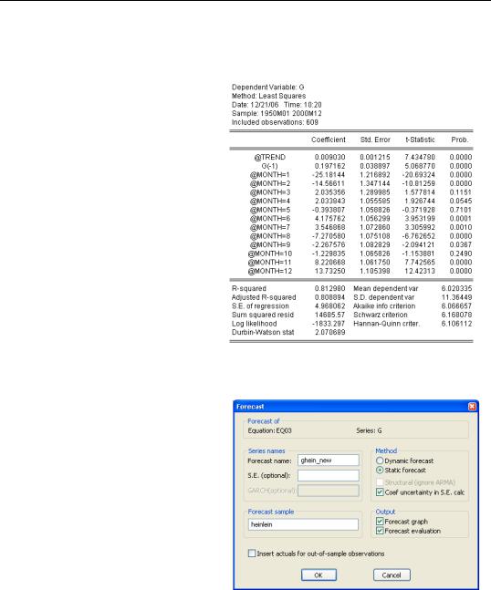
and re-estimate, we find much smaller seasonal effects and a much higher R2 in the TURTLEDOVE world than there was according to HEROTODUS.
Glance back at the data plot which opened the chapter. It shows an enormous increase in currency holdings right before the turn of the millennium and a huge drop immediately thereafter. This means that a dynamic forecast starting in the beginning of 2000 uses an anomalous value for lagged G, a problem which is carried forward. In contrast, a static forecast should only have difficulty at the beginning of the forecast period, since thereafter actual lagged G picks up non-anom- alous data.
Using this new estimate, shown above to the right, as a basis for a static forecast through the HEINLEIN period, we can set the Forecast dialog to save a new forecast, to plot the forecast and confidence intervals, and to show us a new forecast evaluation.
Forecasting Beneath the Surface—235
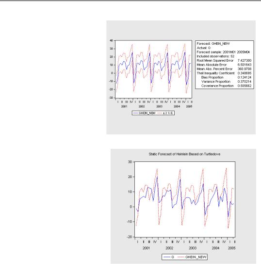
When the Forecast graph and the Forecast evaluation options are both checked, EViews puts the confidence interval graph and statistics together in one window. We’ve definitely gotten a bit of improvement from changing the sample.
One last plot. The seasonal forecast swings are still somewhat larger than the actual seasonal effects, but the forecast is really pretty good for such a simple model.
Forecasting Beneath the Surface
Sometimes the variable you want to forecast isn’t quite the variable on the left of your estimating equation. There are often statistical or economic modeling reasons for estimating a transformed version of the variable you really care about. Two common examples are using logs (rather than levels) of the variable of interest, and using first differences of the variable of interest.

236—Chapter 8. Forecasting
In the example we’ve been using, we’ve taken our task to be forecasting currency growth. If you look at the label for our series G (see Label View in Chapter 2, “EViews—Meet Data”), you’ll see it was derived from an underlying series for the level of currency, CURR, using the command “series g=1200*dlog(curr)”. Since the function dlog takes first differences of logarithms, we actually made both of the transformations just mentioned.
Instead of forecasting growth rates, we could have been asked to forecast the level of currency. In principle, if you know today’s currency level and have a forecast growth rate, you can forecast next period’s level by adding projected growth to today’s level. In practice, doing this can be a little hairy because for more complicated functions it’s not so easy to work backward from the estimated function to the original variable, and because forecast confidence intervals (see below) are nonlinear. Fortunately, EViews will handle all the hard work if you’ll cooperate in one small way:
•Estimate the forecasting equation using an auto-series on the left in place of a regular series.
As a regular series, the information that G was created from “g=1200*dlog(curr)” is a historical note, but there isn’t any live connection. If we use an auto-series, then EViews understands—and can work with—the connection between CURR and the auto-series. We could use the following commands to define an auto-series and then estimate our forecasting equation:
frml currgrowth=1200*dlog(curr)
ls currgrowth @trend currgrowth(-1) @expand(@month)
Forecasting Beneath the Surface—237
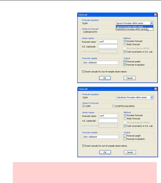
When we hit  in the equation window, we get a Forecast dialog that looks just a little different. The default choice in the dropdown menu is Ignore formulae within series, which means to forecast the auto-series, currency growth in this case.
The alternative choice is Substitute formulae within series. Choose this option and you’re offered the choice of forecasting either the underlying series or the auto-series. We’ve chosen to forecast the level of currency (and set the forecast sample to match the forecast sample in the previous example).
Hint: If you use an expression, for example “1200*dlog(curr)”, rather than a named auto-series as the dependent variable, you get pretty much the same choices, although the dialogs look a little different.