


228—Chapter 8. Forecasting
Dynamic Versus Static Forecasting
Our currency data ends in April 2005. To forecast past that date we need to know the value for @TREND (no problem), which month we’re forecasting for (no problem), and the value of currency growth in the month previous to the forecast month (maybe a problem). It’s this lagged dependent variable that presents a problem/opportunity. If we’re forecasting for May 2005, we’re okay because we know the April value. But for June or later we don’t have the lagged value of currency growth.
A static forecast uses the actual values of the explanatory variables in making the forecast. In our example, we can make static forecasts through May 2005, but no later.
A dynamic forecast uses the forecast value of lagged dependent variables in place of the actual value of the lagged dependent variables. If we start a forecast in May 2005, the dynamic forecast gˆ 2005m5 is identical to the static forecast. Both use g2005m4 as an explanatory variable. The dynamic forecast for June uses gˆ 2005m5 . The static forecast can’t be computed because g2005q5 isn’t known.
Hint: The “^” makes all the difference here. We always have gˆ t – 1 because that’s the number we forecast in period t – 1 . We’re just “rolling the forecasts forward.” In contrast, once we’re more than one period past the end of our data sample gt – 1 is unknown.
The Role of the Forecast Sample
In practice, the difference between static and dynamic forecasting depends on both data availability and the specification of the forecast sample.
Hint: The data used for the explanatory variables in either static or dynamic forecasting is not in any way affected by the sample period used for equation estimation.
Static forecasting uses values of explanatory variables from the forecast sample. If any of them are missing for a particular date, then nothing gets forecast for that date.
Dynamic forecasting pretends that you don’t have any information about the dependent variable during the period covered by the sample forecast—even when you do have the relevant data. In the first period of the forecast sample, EViews uses the actual lagged dependent variables since these actual values are known. In the second period, EViews pretends it doesn’t know the value of the lagged dependent variable and uses the value that it had just forecast for the first period. In the third period, EViews uses the value forecast for the second period. And so on. One of the nice things about dynamic forecasting is that the fore-

Sample Forecast Samples—229
casts roll as far forward as you want—assuming, of course, that the future values of the other right-hand side series are also known.
Mea-very-slightly-culpa: If you’ve been reading really, really closely you may have noticed that the forecast for November 2004 in the graph shown in Just Push the Forecast Button doesn’t match the forecast in the table in Theory of Forecasting. The former was a dynamic forecast (because that’s the EViews default) and the latter was a static forecast (because that’s easier to explain).
Static Versus Dynamic in Practice
Static versus dynamic forecasting are used to simulate answers to two different questions.
Suppose in the future you are going to be tasked with forecasting next month’s currency growth. When the date arrives you’ll have all the necessary data to do a static forecast even though you don’t have the data now. Doing a static forecast now simulates the process you’ll be carrying out later.
In contrast, suppose you are going to be tasked with forecasting currency growth over the next 12 months. When the date arrives you’ll have to do a dynamic forecast. Doing a dynamic forecast now simulates the process you’ll be carrying out later.
One last practical detail. You instruct EViews to do a static or dynamic forecast by picking the appropriate radio button in the Method field of the Forecast dialog. Alternatively, the command fit produces a static forecast and the command forecast produces as dynamic forecast, as in:
forecast gf
Hint: The Structural (ignore ARMA) option isn’t relevant, in fact is grayed out, unless your equation has ARMA errors. See Forecasting in Chapter 13, “Serial Correlation— Friend or Foe?”
Sample Forecast Samples
To check how well your forecasting model works, you want to compare forecasts with what actually happens. One option is to wait until the future arrives and see how things turned out. But the standard procedure is to simulate data arrival by dividing your data sample into an artificial “history” and an artificial “future.” Our monthly currency data runs from 1917 through 2005. We’ll call the complete sample WHOLERANGE; treat most of the period as “history,” HERODOTUS; and reserve the last few years for a “future history,” HEINLEIN. If an equation estimated over HERODOTUS does a good job of forecasting HEINLEIN, then we
230—Chapter 8. Forecasting
can have some confidence that we can re-estimate over WHOLERANGE and then forecast out into the yet-unseen real future:
sample wholeRange @all
sample Herodotus @first 2000
sample Heinlein 2001 @last
’int not intended for Americans: Unless you were born in earshot of Bow bells, in which case it’s ’oleRange, ’erodotus, and ’einlein—not that h’EViews will h’understand.
Using the command line, we create our forecasts with:
smpl herodotus
ls g @trend g(-1) @expand(@month) smpl heinlein
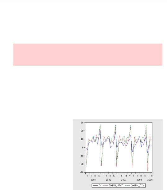
fit ghein_stat forecast ghein_dyn
plot g ghein_stat ghein_dyn
After a little touch up, our graph looks like this. The static and dynamic forecasts look similar and track actual currency growth well. So using this model to forecast the real future seems promising.
Facing the Unknown—231
Setting the Sample in the Forecast Dialog
The forecast dialog can be used if you prefer it to typing commands. Enter the forecast sample, HEINLEIN, in the Forecast sample field. By default, Insert actuals for out-of- sample observations is checked. Under the default, EViews inserts observed G into GHEIN_DYN for data points that aren’t included in the HEINLEIN sample. Uncheck this box to have NAs inserted instead. The advantage of inserting actuals is that it sometimes makes for a prettier plot of the forecast values. The
advantage of inserting NAs is that you won’t accidentally think you forecasted the values outside HEINLEIN.
Facing the Unknown
So far, we’ve forecast a number for a particular date—a point forecast. There is always some degree of uncertainty around this point forecast. Assuming our model is correctly specified, such uncertainty derives from two sources: coefficient uncertainty and error uncertainty. Our forecast for date t is yˆ t = aˆ + bˆ xt while the actual value of the series
we’re forecasting will be yt = a + bxt + ut . The forecast error will be
yt – yˆ t = [(a – aˆ ) + (b – bˆ )xt ] + ut . The term in square brackets is the source of coefficient uncertainty. The error term at the forecast date, ut , causes error uncertainty. If you enter a name next to S.E. (optional) in the Forecast dialog, EViews will save the standard error of the forecast distribution in a series.
It’s not unusual to ignore coefficient uncertainty in evaluating a forecast. If you want to exclude the effect of coefficient uncertainty, uncheck Coef uncertainty in S.E. calc in the dialog.