

Chapter 8. Forecasting
Prediction is very difficult, especially about the future. -Niels Bohr
Think what an easier time Bohr would have had if he’d had EViews, instead of just a Nobel prize in physics!
Truth-be-told, the design of a good model on which to base a forecast can be “very difficult,” indeed. EViews’ role is to handle the mechanics of producing a forecast—it’s up to the researcher to choose the model on which the forecasts are based. We’ll start off with an example of just how remarkably easy the mechanics are, and then go over some of the more subtle issues more slowly.
Just Push the Forecast Button
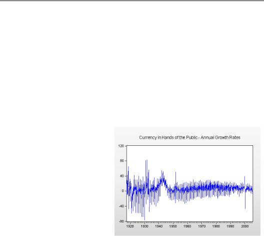
Our goal is to forecast the growth rate of currency in the hands of the public, G. (You can find “currency.wf1” at the EViews website.) A line graph of the data in the series G appears to the right.
For this example, we’re going to
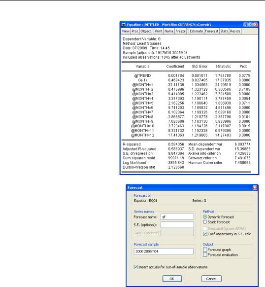
model currency growth as a linear function of a time trend, lagged currency growth, and a different constant for each month of the year. We need to estimate an equation for this model before we can make a forecast. Here’s the relevant command:
ls g @trend g(-1) @expand(@month)
224—Chapter 8. Forecasting
The estimation results look fine.
Now, to produce a forecast, push the  button.
When the Forecast dialog opens, uncheck Forecast graph and Forecast evaluation. (We’ll talk about these later.) Set the Forecast sample at the lower right to 2000 through the end of the sample. Hit  .
.
You’re done. The forecasts for G are stored in the series GF.
Theory of Forecasting—225
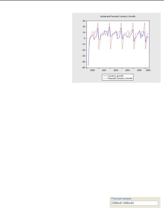
To see how well we did, let’s plot actual and forecast currency growth together. Pretty good forecasting, no? Perhaps leaning a little too heavily on seasonal fluctuations, but basically pretty satisfactory.
You now know almost everything you need to forecast in EViews. (We told you the mechanics were easy!)
Theory of Forecasting
Let’s review a little forecasting theory and then see where EViews fits in.
There are three steps to making an accurate forecast:
1.Formulate a sound model for the variable of interest.
2.Estimate the parameters attached to the explanatory variables.
3.Apply the estimated parameters to the values of the explanatory variables for the forecast period.
Let’s call the variable we’re trying to forecast y . Suppose that a good way to explain y is with the variable x and that we’ve decided on the model:
yt = a + bxt + ut ,
where in our opening example, x would represent the time trend, lagged currency growth, etc.
Choosing a form for the model was Step 1. Now gather data on for periods
t = 1…T and use one of EViews’ myriad estimation techniques—perhaps least squares, but perhaps another method—to assign numerical estimates, aˆ and bˆ , to the parameters in the model. You can see the estimated parameters in the equation EQ01 above. That was Step 2.
Finally, let’s say that we want to forecast yt at all the dates t starting at TF and continuing through TL . This is the forecast sample, which is to say the entry marked Forecast sample in the lower left part of the Forecast dialog. Our forecast will be:

226—Chapter 8. Forecasting
yˆ t = aˆ + bˆ xt
In other words, Step 3 consists of multiplying each estimated coefficient from Step 2 by the relevant x value in the forecast period, and then adding up the products. The formalism will turn out to be convenient for our discussion below. For now, let’s use the example we’ve been working with to forecast for November 2004.
The “x ” variables in our equation are a time trend, growth the previous month, and a set of dummy (0/1) variables for the month. To forecast, we need the values of each x variable and the estimated coefficient attached to that variable. The required data appear in the following table.
Table 3
x |
Estimated |
Value of x |
Product |
|
Parameters |
|
|
|
|
|
|
|
|
|
|
@TREND |
0.001784 |
1047 |
1.87 |
|
|
|
|
G2004m10 |
0.469423 |
3.4105 |
1.60 |
@MONTH=11 |
8.321732 |
1.0 |
8.32 |
|
|
|
|
ˆ |
|
|
11.79 |
G2004m11 |
|
|
|
G2004m11 |
|
|
12.42 |
forecast error |
|
|
0.63 |
|
|
|
|
When you click the  button EViews does the same calculation—just faster and with some extra doo-dads available in the output.
In-Sample and Out-Of-Sample Forecasts
In carrying out Step 3, there’s an implicit issue that deserves explicit attention. Before we could start multiplying parameters times x variables in the table above we needed to know the values of x in the forecast period.
In our table, the value of @TREND is 1047, the month number in our data for November 2004. (We cheated and looked the number up by giving the command show @trend, which opens a spreadsheet view of @TREND.) The November value of lagged currency growth is the October currency growth number, 3.4105. And @MONTH=11 always equals 1.0 in November.
Suppose we had estimated a better model that used the inflation rate as an explanatory variable? To carry out the forecast, we would need to know the November 2004 inflation rate. But suppose we were forecasting for November 2104? There’s no way we’re going to be able to plug in the right value of inflation 100 years from now. No inflation rate, no forecast.
The cardinal rule of practical forecasting is:

Theory of Forecasting—227
•Know the values of the explanatory variables during the forecast period—or know a way to forecast the required explanatory variables.
We’ll return to “know a way to forecast the required explanatory variables” in the next section.
Knowing that you will have to deal with the cardinal rule in Step 3 sometimes influences what you do in Step 1. The corollary to the practical rule of forecasting is:
•There’s not much point in developing a great model for forecasting if you won’t be able to carry out the forecast because you don’t know the required future values of all of the explanatory variables.
This aspect of model development is important, but doesn’t really have anything to do with using EViews—so we’ll leave it at that.
In our example above, we didn’t have to face this issue because we were making an in-sam- ple forecast; a forecast where TL ≤ T . We knew the values of all the explanatory variables for the forecast period because the forecast period was a subset of the estimation period. Insample forecasting has two advantages: you always have the required data, and you can check the accuracy of your forecast by comparing it to what actually happened. We forecast 11.79 percent currency growth for November 2004. Currency growth was actually 12.42 percent, so the forecast error was a bit above a half a percent. Not too bad.
The alternative to in-sample forecasting is out-of-sample forecasting, where TF > T . You have to obey the cardinal rule when forecasting out-of-sample. And sometimes, that’s a problem because you lack out-of-sample values of some of the x variables. What’s more, the history of forecasting is replete with examples that work well in-sample but fall apart out-of-sample. A common compromise is to reserve part of the data by not including it in the estimation sample, effectively pretending that the reserve sample is in the future. Then conduct an out-of-sample forecast over the reserved sample, taking advantage of the known values of the explanatory variables and observed outcomes. We’ll walk through this sort of exercise in Sample Forecast Samples.
One other disadvantage of in-sample forecasting: It’s really hard to get someone to pay you to forecast something that’s already happened.
Practical hint: If you’re like the author, you usually set up the range of your EViews workfile to coincide with your data sample. Then, when I forecast out-of-sample, I get an error message saying the forecast sample is out of range. When this happens to you, just double-click Range in the upper panel of the workfile window to extend the range to the end of your forecasting period.