112—Chapter 4. Data—The Transformational Experience

Many-To-One Mappings

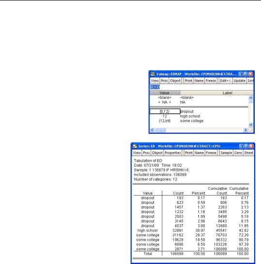
Value maps can be used to group a range of codes for the purpose of display. Instead of a single value in the value map, enter a range in parentheses. For example “(-inf, 12)” specifies all values less than 12. Parentheses are used to specify open intervals, square brackets are used for closed intervals. So “(-inf, 12]” is all values less than or equal to 12.

The series ED in “CPSMAR2004Extract.wf1” measures education in years. We could use the value map shown to the right to group education into three displayed values.

The many-to-one mapping is only for display purposes. If we analyze the data, all the underlying categories are still there. For example, here’s a tabulation of ED. Everyone with less than a high school education is labeled “dropout,” but they’re still tabulated in separate categories according to the years of education they’ve had. That’s why we see seven “dropout” rows on the right.

Relative Exotica

EViews has lots of functions for transforming data. You’ll never need most of these functions, but the one you do need you’ll need bad.

Stats-By

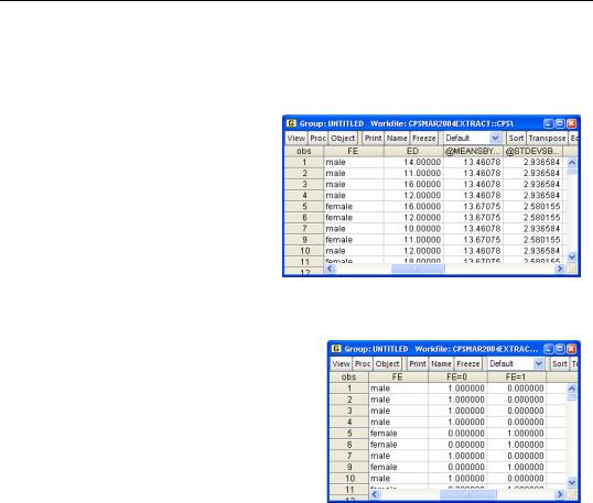
We met several data summary functions such as @mean above in the section Functions Are Where It’s @. Sometimes one wants a summary statistic computed by group. We might want a series that assigned the mean education for women to women and the mean education for men to men. This is accomplished with the Stats-By family of functions: @meansby(x,y),

@mediansby(x,y), etc. (See the Command and Programming Reference for more func-

Relative Exotica—113

tions.) These functions summarize the data in X according to the groups in Y. (Optionally, a sample can be used as a third argument.) Thus the command:

show fe ed @meansby(ed,fe) @stdevsby(ed,fe)

shows gender and years of education followed by the mean and standard deviation of education for women if the individual is female, and the mean and standard deviation of education for men if the individual is male.

Expand the Dummies

The @expand function isn’t really a data transformation function at all. Instead, @expand(x) creates a set of temporary series. One series is created for each unique value of X and the value of a given series is 1 for observations where X equals the corresponding value. For example, @expand(fe) creates two series in the command:

show fe @expand(fe)

If you give @expand more than one series as

an argument, as in @expand(x,y,z), series are created for all possible combinations of the values of the series.

The primary use of @expand is as part of a regression specification, where it generates a complete set of dummy variables. Because it’s often desirable to omit one series from the complete set, @expand can take an optional last argument, @dropfirst or @droplast. The former omits the first category from the set of series generated and the latter omits the last category. (For more detail, see the Command and Programming Reference).

@expand can also be used in algebraic expressions, with each resulting temporary series being inserted in the expression in turn. The command,

ls lnwage c ed*@expand(fe)

is equivalent to:

ls lnwage c ed*(fe=0) ed*(fe=1)

114—Chapter 4. Data—The Transformational Experience

and estimates separate returns to education for men and women.

Statistical Functions

Uniform and standard normal random number generators were described earlier in the chapter. EViews supplies families of statistical functions organized according to specific probability distributions. A function name beginning with “@r” is a random number generator, a name beginning with “@d” evaluates the probability density function (also called the “pdf”), a name beginning with “@c” evaluates the cumulative distribution function (or “cdf”), and a name beginning with “@q” gives the quantile, or inverse cdf. In each case, the @-sign and initial letter are followed by the name of the distribution.

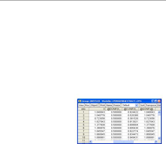
As an example, the name used for the uniform distribution is “unif.” So @runif(a,b) generates random numbers distributed uniformly between A and B. (This means that @rnd is a synonym for @runif(0,1).) We can make up an example with:

series x = @runif(0,2)

show x @dunif(x,0,2) @cunif(x,0,2) @qunif(@cunif(x,0,2),0,2)

which randomly resulted in the data shown to the right. The first column, X, is a random number randomly distributed between 0 and 2. The second column gives the pdf for X, which for this distribution always equals 0.5. The third column gives the cdf. Just for fun, the last column reports the inverse cdf of the cdf, which is the original X, just as it should be.

A variety of probability distributions are discussed in the Command and Programming Reference. Probably the most commonly used are “norm,” for standard normal, and “tdist,” for Student’s t. Here are a few examples:

=@qtdist(.95, 30) = 1.69726

=@qtdist(0.05/2, 30) = -2.04227

=@qnorm(.025) = -1.95996

Quick Review

Data in EViews can be either numbers or text. A wide set of data manipulation functions are available. In particular, the “expected” set of algebraic manipulations all work as expected. You can use numbers to conveniently represent dates. EViews also provides control over the