

106—Chapter 4. Data—The Transformational Experience
Can We Have A Date?
Technically, EViews doesn’t have a “date type.” Instead, EViews has a bunch of tools for interpreting numbers as dates. If all you do with dates is look at them, there’s no need to understand what’s underneath the hood. This section is for users who want to be able to manipulate date data.
The key to understanding EViews’ representation of dates is to take things one day at a day:
•An observation in a “date series” is interpreted as the number of days since Monday, January 1, 0001 CE.
Date series are manipulated in three ways: you can control their display in spreadsheet views, you can convert back and forth between date numbers and their text representation, and you can perform date arithmetic.
Date Displays
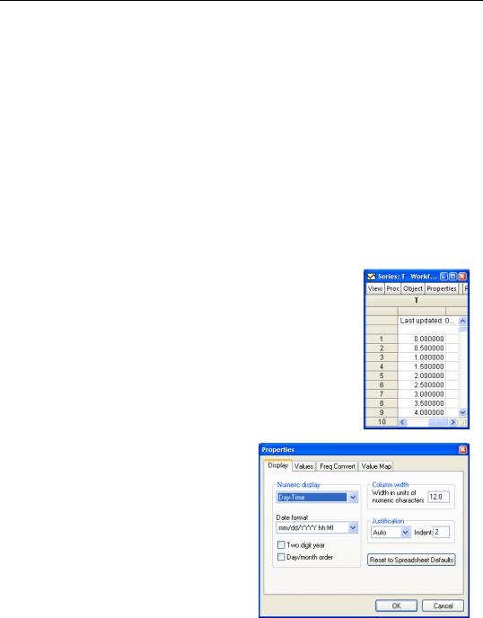
Open a series T=0, 0.5, 1, 1.5, 2,… and you get the standard spreadsheet view.
Use the  button to bring up the Properties dialog. Choose Day-Time to change the display to treat the numbers as dates showing both day and time.
Can We Have A Date?—107
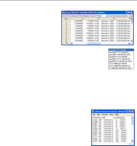
The display changes as shown to the right. Notice that fractional parts of numbers correspond to a fraction of a day. Thus 1.5 is 12 noon on the second day of the Common Era. Two Day and Time formats are also shown by way of illustration.
The Date format dropdown menu provides a variety of date display formats.
Date to Text and Back Again
“January 1, 1999” is more easily understood by humans than is its date number representation, “729754.” On the other hand, comput-
ers prefer to work with numbers. A variety of functions translate between numbers interpreted as dates and their text representation.
The function @datestr(x[,fmt]) translates the number in X into a text string. A second optional argument specifies a format for the date. As examples, @datestr(731946) produces “1/1/2005”; @datestr(731946,"Month dd, yyyy") gives “January 1, 2005”; and @datestr(731946,"ww") produces a text string representation of the week number, “6.” More date formats are discussed in the User’s Guide.
The inverse of @datestr is @dateval, which converts a string into a date number. @dateval is particularly useful when you’ve read in text representing dates and want a numerical version of the dates so that you can manipulate them. The file “SPClose Text excerpt.txt” has the closing prices for the S&P 500 for the first few days of 2005. Reading this into EViews gives a numeric series for SP500CLOSE and an alpha series for CLOSEDATE. The command:
series tradedate = @dateval(closedate)
gives a numerical date series which is then available for further manipulation.
@makedate translates ordinary numbers into date numbers, for example @makedate(1999, "yyyy") returns 729754, the first day in 1999. The format strings used for the last argument of @makedate are also discussed in the User’s Guide.

108—Chapter 4. Data—The Transformational Experience
The workfile “SPClose2005.wf1” includes S&P 500 daily closing prices (SP500CLOSE) on a given YEAR, MONTH, and DAY. To convert the last three into a usable date series use the command:
series tradedatenum = @makedate(year,month,day,"yyyy mm dd")
To turn these into a series that looks like ‘“January 3, 2005”’ (etc.), use the command:
alpha tradedate = """" + @datestr(tradedatenum,"Month dd, yyyy") +
""""
In this command the four quotes in a row are interpreted as a quote opening a string (first quote), two quotes in a row which stand for one quote inside the string (middle two quotes), and a quote closing the string (last quote). It takes all four quotes to get one quote embedded in the string.
Date Manipulation Functions
Since dates are measured in days, you can add or subtract days by, unsurprisingly, adding or subtracting. For example, the function @now gives (the number representing) the current day and time, so @now + 1 is the same time tomorrow.
The functions @dateadd(date1,offset[,units_string]) and
@datediff(date1,offset[,units_string]) add and subtract dates, allowing for different units of time. The units_string argument specifies whether you want arithmetic to be done in days (“dd”), weeks (“ww”), etc. (See the User’s Guide for information on “etc.”)
@dateadd(@now,1,"dd") is this time tomorrow, while @dateadd(@date,1,"ww") is this time on the same day next week.
Suppose we want to compute annualized returns for our 2005 S&P closing price data. We can compute the percentage change in price from one observation to the next with,
series pct_change = (sp500close-sp500close(-1))/sp500close(-1)
or with the equivalent built-in command @pch:
series pct_change = @pch(sp500close)
To annualize a daily return we could multiply by 365. (Or we could use the more precise formula that takes compounding into account, (1 + pct_change)365 – 1 ). But some of our
returns accumulated over a weekend, and arguably represent three days’ earnings. Taking into account that the number of days between observations varies, we can annualize the return with:
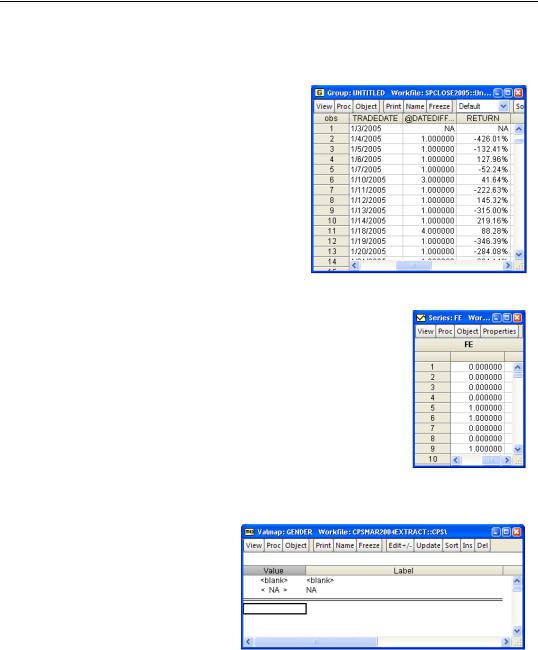
series return = (365/@datediff(tradedatenum, tradedate- num(-1),"dd"))*pct_change
Let’s take this apart. The expression ‘@datediff(tradedatenum, tradedatenum(-1),"dd")’ returns the number of days between observations. Usually there’s one day between obser-
What Are Your Values?—109
vations, giving us 365/1. Over an ordinary weekend, the datediff function returns 3, so we annualize by multiplying by 365/3.
Note two things about annualized returns. First, typical daily returns imply very large annual rates of change. In fact, the annual rates are implausible. Second, we’ve captured not only weekends, but also the January 17th closing in honor of Dr. King.
What Are Your Values?
The workfile “CPSMAR2004Extract.wf1” is a cross section of individuals from the Current Population Survey. The series FE codes a person’s gender. As you will remember from early biology lessons, humans have two genders—0 and 1.
Some of us prefer to think of humans as male and female, rather than 0 and 1. EViews uses value maps to translate the appearance of codes into something more pleasant to read. The codes themselves are unchanged—it’s their appearance that’s improved.
To create a new value map named GENDER, use Object/New
Object…/ValMap or type the command:
valmap gender
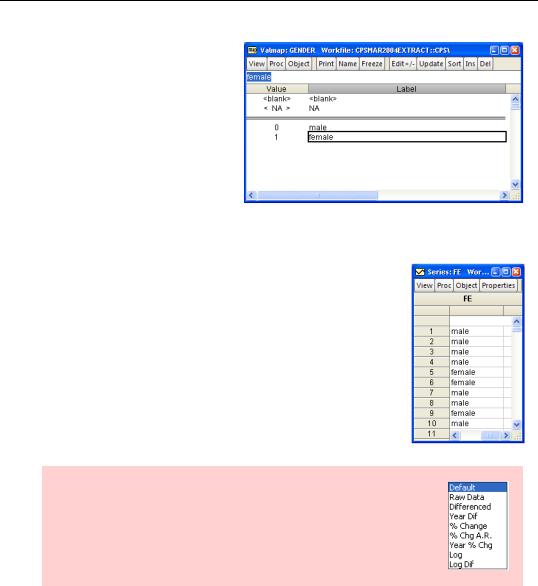
The ValMap editor view pops up showing two columns. Values (0 or 1 in this case) go on the left and the corresponding labels (male, female) go on the right. Two default mappings appear at the top: blanks and NAs are displayed unchanged.
110—Chapter 4. Data—The Transformational Experience
To fill out the value map, enter a list of codes on the left and labels on the right. When you close the valmap window,  is stored in the workfile with an icon that says “map.” (The values can be either numeric or text, and there’s no harm in providing maps for values that aren’t used.) To tell EViews to use the map just created, open the series FE, click the
  button, choose the Value Map tab and type in GENDER.
Displayed FE now uses much friendlier labels.
Hint: If you want to see FE’s underlying codes, switch the display type menu in the series spreadsheet view from Default to Raw Data.
EViews will use the new labels wherever possible. For example, the command:
ls lnwage ed @expand(fe)
What Are Your Values?—111
which regresses a series containing log(wage) on education and
a dummy variable for each gender produces nicely labeled output. (More on the @expand function under Expand the Dummies).
In fact, you can use the value labels in editing a series. (Be sure the Display type menu is set to Default.) EViews checks to see if an entry matches any of the labels in the value map. If so, the corresponding value is entered. If not, the new entry is used directly. As
a consequence, you can use either the label or underlying code to enter a new value—so long as the underlying code hasn’t been used to label some other value.
Hint: Labels in the editor are case sensitive, e.g., “male” translates to 0 but “Male” translates to NA.
Since a value map is just a translation from underlying code to appearance, you’re free to use the same value map for multiple series. To help keep track of which series is using a given value map, the Usage view of a value map shows a list of all the series currently attached.
Hint: EViews doesn’t care what you use for a label. It will cheerfully let you label the number “0” with the value map “1”. Don’t. For further discussion, see Origin of the Species.
Hint: If you load data created in another stat program that has its own version of value maps, EViews will create value maps and correctly hook them up to the relevant series. However, there’s no general method using values in an alpha series as labels in a value map.