

Simple Sample Says—95
Hint: frml is a contraction of “formula.”
To understand named auto-series, it helps to know what EViews is doing under the hood. For an ordinary series, EViews computes the values of the series and stores them in the workfile. For a named auto-series, EViews stores the formula you provide. Whenever the auto-series is referenced, EViews recalculates its values on the fly. A minor advantage of the auto-series is that it saves storage, since the values are computed as needed rather than always taking up room in memory.
The major advantage of named auto-series is that the values automatically update to reflect changes in values of series used in the formula. In the example above, if any of the data in Y changes, the values in Y_LESS_MEAN change automatically.
When we get to Chapter 8, “Forecasting,” we’ll learn about a special role that auto-series play in making forecasts.
Simple Sample Says
As you’ve no doubt gathered by now, the statement “Operations are performed on an entire series at a time” is a hair short of being true. The fuller version is:
•Operations are performed on all the elements of a series included in the current sample.
A sample is an EViews object which specifies which observations are to be included in operations. Effectively, you can think of a sample as a list of dates in a dated workfile, or a list of observation numbers in an undated workfile. Samples are used for operational control in two different places. The primary sample is the workfile sample. This sample provides the default control for all operations on series, by telling which observations to include. Specific commands occasionally allow specification of a secondary sample which over-rides the workfile sample.
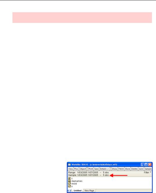
When a workfile is first created, the sample includes all observations in the workfile. The current sample is shown in the upper pane of the workfile window. In this example, the workfile consists of five daily observations beginning on Mon-
day, January 3, 2005 and ending on Friday, January 7, 2005.
Here’s the key concept in specifying samples:
96—Chapter 4. Data—The Transformational Experience
• Samples are specified as one or more pairs of beginning and ending dates.
In the illustration, the pair “1/03/2005 1/07/05” specifies the first and last dates of the sample.
Hint: Above, we used the word “date.” For an undated workfile, substitute “observation number.” To pick out the first ten observations in an undated workfile use the pair “1 10.”
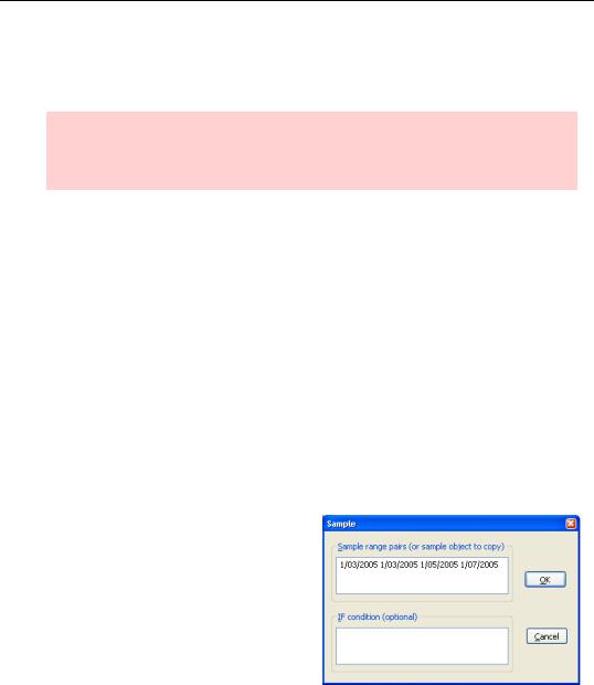
To pick out Monday and Wednesday through Friday, specify the two pairs “1/03/2005 1/03/2005 1/05/2005 1/07/2005.” Notice that we picked out a single date, Monday, with a pair that begins and ends on the same date.
EViews is clever about interpreting sample pairs as beginning and ending dates. In a daily workfile, specifying 2005m1 means January 1 if it begins a sample pair and January 31 if it ends a sample pair. As an example,
smpl 2005m1 2005m1
picks out all the dates in January 2005.
SMPLing the Sample
To set the sample, use the smpl command. (Not the related sample command, which we’ll get to in a second.) The command format is the word smpl, followed by the sample you want used, as in:
smpl 1/03/2005 1/03/2005 1/05/2005 1/07/2005
If you prefer, the menu Quick/Sample… or the  button (which implements the smpl command, not the sample command) brings up the Sample dialog where you can also type in the sample. The dialog is initialized with the current sample for ease of editing.
SMPL Keywords
Three special keywords help out in specifying date pairs. @first means the first date in the workfile. @last means the last date. @all means all dates in the workfile. So two equivalent commands are:
smpl @all
smpl @first @last

Simple Sample Says—97
Arithmetic operations are allowed in specifying date pairs. For example, the second date in the workfile is @first+1. To specify the entire sample except the first observation use:
smpl @first+1 @last
The first ten and last ten observations in the workfile are picked by:
smpl @first @first+9 @last-9 @last
Smpl Splicing
You can take advantage of the fact that observations outside the current sample are unaffected by series operations to splice together a series with different values for different dates. For example, the commands:
smpl @all
series prewar = 1
smpl 1945m09 @last
prewar = 0
smpl @all
first create a series equal to 1.0 for all observations. Then it sets the later observations in the series to 0, leaving the pre-war values unchanged.
Hint: It is a very common error to change the sample for a particular operation and then forget to restore it before proceeding to the next step. At least the author seems to do this regularly.
SMPLing If
A sample specification has two parts, both of which are optional. The first part, the one we’ve just discussed, is a list of starting and ending date pairs. The second part begins with the word “if” and is followed by a logical condition. The sample consists of the observations which are included in the pairs in the first part of the specification AND for which the logical condition following the “if” is true. (If no date pairs are given, @all is substituted for the first part.) We could pick out the last three weekdays with:
smpl if @weekday>=3 and @weekday<=5
We could pick out days in which the NASDAQ closed above 2,100 (remember that the series Y is the NASDAQ closing price) with:
smpl if y>2100
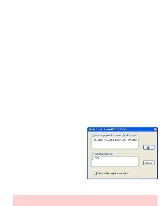
To select the days Monday and Wednesday through Friday in the first trading week of 2005, but only for those days where the NASDAQ closed above 2,100, type:
smpl 1/03/2005 1/03/2005 1/05/2005 1/07/2005 if y>2100
98—Chapter 4. Data—The Transformational Experience
Sample SMPLs
Since the smpl command sets the sample, you won’t be surprised to hear that the sample command sets smpls.
The sample command creates a new object which stores a smpl. In other words, while the smpl command changes the active sample, the sample command stores a sample specification for future use. Sample objects appear in the workfile marked with a  icon. Thus the command:
sample s1 1/03/2005 1/03/2005 1/05/2005 1/07/2005 if y>2100
stores  in the workfile. You can later reuse the sample specification with the command:
smpl s1
remembering that the specification is evaluated when used, not when stored. In fact, there’s an important general rule about the evaluation of sample specifications:
• The sample is re-evaluated every time EViews processes data.
The example at hand includes the clause “if y>2100”. Every time the values in Y change, the set of points included in the sample may change. For example, if you edit Y, changing an observation from 2200 to 2000, that observation drops out of sample S1.
Three Simple SAMPLE & SMPL Tricks
To save the current sample specification, give the command sample or use the menu Object/New Object and pick Sample. Either way, the Sample dialog opens with the current workfile sample as initial values. Immediately hit  to save the current specification in the newly defined sample object.
Remember that the “if clause” in a sample includes observations where the logical condition evaluates to TRUE (1) and excludes observations where the condition evaluates to False (0).
Hint: In a sample “if clause,” NA counts as false.

Simple Sample Says—99
Freezing the current sample
To “freeze” a sample, so that you can reuse the same observations later even if the variables in the sample specification change, first create a variable equal to 1 for every point in the current sample.
series sampledummy = 1
Then set up a new sample which selects those data points for which the new variable equals 1.
sample frozensample if sampledummy
Now any time you give the command:
smpl frozensample
you’ll restore the sample you were using.
Creating dummy variables for selected dates
To create a dummy (zero/one) variable that equals one for certain dates and zero for others, first save a sample specification including the desired dates. Later you can include the sample in a series calculation, taking advantage of the fact that in such a calculation EViews evaluates the sample as 1 for points in the sample and 0 for points outside. Try deconstructing the following example.
sample s2 @first+1 @last if y=y(-1)
smpl @all
series sameyasprevious = y*s2 - 999*(1-s2)
Got it? The first line defines S2 as holding a sample specification including all observations for which Y equals its own lagged value. The second line sets the sample to include the entire workfile range. The third line creates a new series named SAMEYASPREVIOUS which equals Y if Y equals its own lagged value and -999 otherwise. The trick is that the sample S2 is treated as either a 1 or a 0 in the last line.
Nonsample SMPLs
Each workfile has a current sample which governs all operations on series—except when it doesn’t. In other words, some operations and commands allow you to specify a sample which applies just to that one operation. For these operations, you write the sample specification just as you would in a smpl command. In some cases, the string defining the sample needs to be enclosed in quotes.
We’ve already seen one such example. The function @mean accepts a sample specification as an optional second argument. Following along from the preceding example, we could compute:
smpl @all