

Chapter 4. Data—The Transformational Experience
It’s quite common to spend the greater part of a research project manipulating data, even though the exciting part is estimating models, testing hypotheses, and forecasting into the future. In EViews the basics of data transformation are quite simple. We begin this chapter with a look at standard algebraic manipulations. Then we take a look at the different kinds of data—numeric, alphabetic, etc.—that EViews understands. The chapter concludes with a look at some of EViews’ more exotic data transformation functions.
Your Basic Elementary Algebra
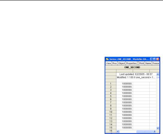
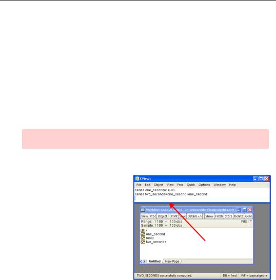
The basics of data transformation in EViews can be learned in about two seconds. Suppose we have a series named ONE_SECOND that measures—in microseconds—the length of one second. (You can download the workfile “BasicAlgebra.wf1”, from the EViews website.) To create a new EViews series measuring the length of two seconds, type in the command pane:
series two_seconds = one_second + one_second
84—Chapter 4. Data—The Transformational Experience
Deconstructing Two Seconds Construction
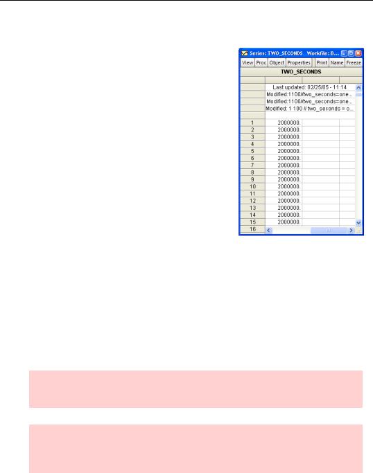
The results of the command are shown to the right. They’re just what one would expect. Let’s deconstruct this terribly complicated example. The basic form of the command is:
•the command name series, followed by a name for the new series, followed by an “=” sign, followed by an algebraic expression.
A number of EViews’ “cultural values” are implicitly invoked here. Let’s go though them one-by-one:
•Operations are performed on an entire series at a time.
In other words, the addition is done for each observation at the same time. This is the general rule but we’ll see two variants a little later, one involving lags and one involving samples.
•The “=” sign doesn’t mean “equals,” it means
copy the values on the right into the series on the left.
This is standard computer notation, although not what we learned “=” meant in school. Note that if the series on the left already exists, the values it contains are replaced by those on the right. This allows for both useful commands such as:
series two_seconds = two_seconds/1000 'change units to milliseconds
and also for some really dumb ones:
series two_seconds = two_seconds-two_seconds 'a really dumb command
Hint: EViews regards text following an apostrophe, “'”, as a comment that isn’t processed. “'a really dumb command” is a note for humans that EViews ignores.
Hint: There’s no Undo command. Once you’ve replaced values in a series—they’re gone! Moral: Save or SaveAs frequently so that if necessary you can load back a premistake version of the workfile.
Your Basic Elementary Algebra—85
•The series command performs two logically separate operations. It declares a new series object, TWO_SECONDS. Then it fills in the values of the object by computing ONE_SECOND+ONE_SECOND
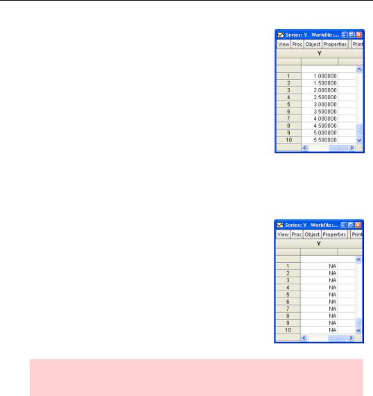
We could have used two commands instead of one:
series two_seconds
creates a series in the workfile named TWO_SECONDS initialized with NAs. We could then type:
two_seconds = one_second + one_second
Once a series has been created (or “declared,” in computer-speak) the command name series is no longer required at the front of a data transformation line— although it doesn’t do any harm.
Hint: EViews doesn’t care about the capitalization of commands or series names.
Some Typing Issues
The command pane provides a scrollable record of commands you’ve typed. You can scroll back to see what you’ve done. You can also edit any line (including using copy-and- paste to help on the editing.) Hit Enter and EViews will copy the line containing the cursor to the bottom of the command pane and then execute the command.
You may wish to use (CTRL+UP) to recall a list of previous commands in the order they were entered. The last
command in the list will be entered in the command window. Holding down the CTRL key and pressing UP repeatedly will display the prior commands. Repeat until the desired command is recalled for editing and execution.
If you’ve been busy entering a lot of commands, you may press (CTRL+J) to examine a history of the last 30 commands. Use the UP and DOWN arrows to select the desired command and press ENTER, or double click on the desired command to add it to the command window. To close the history window without selecting a command, click elsewhere in the command window or press the Escape (ESC) key.
86—Chapter 4. Data—The Transformational Experience
The size of the command pane is adjustable. Use the mouse to grab the separator at the bottom of the command pane and move it up or down as you please. You may also drag the command window to anywhere inside the EViews frame. Press F4 to toggle docking, or click on the command window, depress the right-mouse button and select Toggle Command Docking.
You can print the command pane by clicking anywhere in the pane and then choosing File/Print. Similarly, you can save the command pane to disk (default file name “command.log”) by clicking anywhere in the pane and choosing File/Save or File/SaveAs….
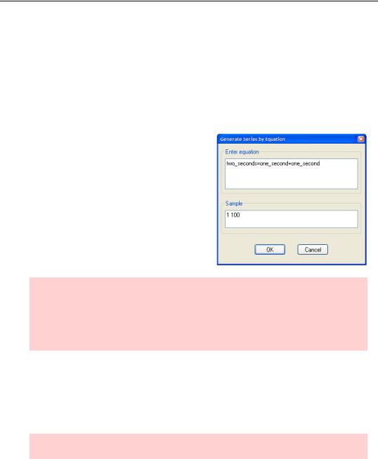
Some folks have a taste for using menus rather than typing commands. We could have created TWO_SECONDS with the menu Quick/Generate Series…. Using the menu and Generate Series by Equation dialog has the advantage that you can restrict the sample for this one operation without changing the workfile sample. (More on samples in the next section.) There’s a small disadvantage in that, unlike when you type directly in the command pane, the equation doesn’t appear in the command pane—so you’re left without a visual record.
Deprecatory hint: Earlier versions of EViews used the command genr for what’s now done with the distinct commands series, alpha, and frml. (We’ll meet the latter two commands shortly.) Genr will still work even though the new commands are preferred. (Computer folks say an old feature has been “deprecated” when it’s been replaced by something new, but the old feature continues to work.)
Obvious Operators
EViews uses all the usual arithmetic operators: “+”, “-”, “*”, “/”, “^”. Operations are done from left to right, except that exponentiation (“^”) comes before multiplication (“*”) and division, which come before addition and subtraction. Numbers are entered in the usual way, “123” or in scientific notation, “1.23e2”.
Hint: If you aren’t sure about the order of operations, (extra) parentheses do no harm.
EViews handles logic by representing TRUE with the number 1.0 and FALSE with the number 0. The comparison operators “>”, “<“, “=”, “>=” (greater than or equal), “<=” (less than or equal), and “<>” (not equal) all produce ones or zeros as answers.
Your Basic Elementary Algebra—87
Hint: Notice that “=” is used both for comparison and as the assignment operator— context matters.
EViews also provides the logical operators and, or, and not. EViews evaluates arithmetic operators first, then comparisons, and finally logical operators.
Hint: EViews generates a 1.0 as the result of a true comparison, but only 0 is considered to be FALSE. Any number other than 0 counts as TRUE. So the value of the expression 2 AND 3 is TRUE (i.e., 1.0). (2 and 3 are both treated as TRUE by the AND operator.)
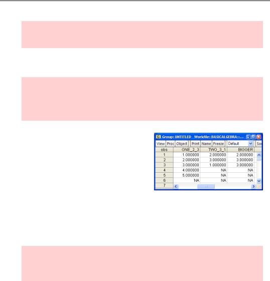
Using 1 and 0 for TRUE and FALSE sets up some incredibly convenient tricks because it means that multiplying a number by TRUE copies the number, while multiplying by FALSE gives nothing (uh, zero isn’t really “nothing,” but you know what we meant). For example, if the series ONE_2_3 and TWO_3_1 are as shown, then the command:
series bigger = (one_2_3>=two_3_1)*one_2_3 + (one_2_3<two_3_1)*two_3_1
picks out the values of ONE_2_3 when ONE_2_3 is larger than TWO_3_1
( 1 × ONE_2_3 + 0 × TWO_3_1) and the values of TWO_3_1 when TWO_3_1 is larger ( 0 × ONE_2_3 + 1 × TWO_3_1) .
Na, Na, Na: EViews code for a number being not available is NA. Arithmetic and logical operations on NA always produce NA as the result, except for a few functions specially designed to translate NAs. NA is neither true nor false; it’s NA.
The Lag Operator
Reflecting its time series origins a couple of decades back, EViews takes the order of observations seriously. In standard mathematical notation, we typically use subscripts to identify one observation in a vector. If the generic label for the current observation is yt , then the previous observation is written and the next observation is written . When there isn’t any risk of confusion, we sometimes drop the t. The three observations might be written y–1, y, y+1 . Since typing subscripts is a nuisance, lags and leads are specified in EViews by following a series name with the lag in parentheses. For example, if we have a series
88—Chapter 4. Data—The Transformational Experience
named Y, then Y(-1) refers to the series lagged once; Y(-2) refers to the series lagged twice; and Y(1) refers to the series led by one.
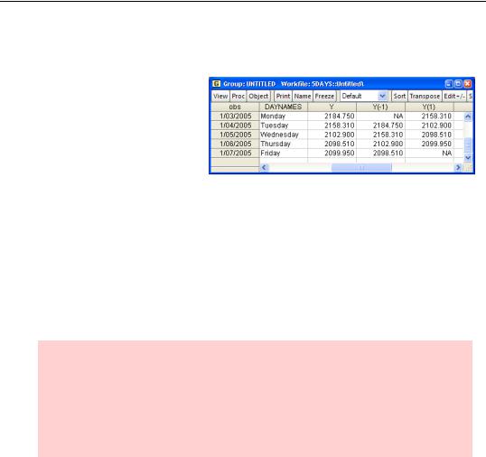
As an illustration, the workfile “5Days.wf1” contains a series Y with NASDAQ opening prices for the first five weekdays of 2005. Looking at Tuesday’s data you’ll see that the value for Y(-1) is Monday’s opening price and the value for Y(1) is
Wednesday’s opening price. Y(-1) for Monday and Y(1) for Friday are both NA, because they represent unknown data—the opening price on the Friday before we started collecting data and the opening price on the Monday after we stopped collecting data, respectively.
The group shown above was created with the EViews command:
show daynames y y(-1) y(1)
If we wanted to compute the percentage change from the previous day, we could use the command:
series pct_change = 100*(y-y(-1))/y(-1)
Hint: In a regularly dated workfile, “5Days.wf1” for example, one lag picks up data at t – 1 . In an undated or an irregularly dated workfile, one lag simply picks up the preceding observation—which may or may not have been measured one time period earlier.
Put another way, in a workfile holding data for U.S. states in alphabetical order, one lag of Missouri is Mississippi.
The “Entire Series At A Time” Exception For Lags
A couple of pages back we told you that EViews operates on an entire series at a time. Lags are the first exception. When the expression on the right side of a series assignment includes lags, EViews processes the first observation, assigns the resulting value to the series on the left, and then processes the second observation, and so on. The order matters because the assignment for the first observation can affect the processing of the second observation.
Consider the following EViews instructions, ignoring the smpl statements for the moment.
smpl @all
series y = 1
smpl @first+1 @last
y = y(-1) + .5
Your Basic Elementary Algebra—89
The first assignment statement sets all the observations of Y to 1. As a consequence of the second smpl statement (Smpl limits operations to a subset of the data; more on smpl in the section Simple Sample Says), the second assignment statement begins with the second observation, setting Y to the value of the first observation (Y(-1)) plus .5 (1.0+0.5). Then the statement sets the third observation of Y to the value of the second observation (Y(-1)) plus .5 (1.5+0.5). Contrast this with processing the entire series at a time, adding .5 to each original lagged observation (setting all values of Y to 1.5)—which is what EViews does not do.
Now we’ll unignore the smpl statements. If we’d simply typed the commands:
series y = 1
y = y(-1) + .5
the first assignment would set all of Y to 1. But the second statement would begin by adding the value of the zeroth observation (Y(-1))—oops, what zeroth observation? Since there is no zeroth observation, EViews would add NA to 0.5, setting the value of the first Y to NA. Next, EViews would add the first observation to 0.5, this time setting the second Y to NA+0.5. We would have ended up with an entire series of NAs.
Our original use of smpl statements to avoided propagating NAs by having the first lagged value be the value of the first observation, which was 0—as we intended.
Moral: When you use lagged variables in an equation, think carefully about whether the lags are picking up the observations you intend.
Functions Are Where It’s @
EViews function names mostly begin with the symbol “@.” There are a lot of functions which are documented in the Command and Programming Reference. We’ll work through some of the more interesting ones below in the section Relative Exotica. Here, we look at the basics.
Several of the most often used functions have “reserved names,” meaning these functions don’t need the “@” sign and that the function names cannot be used as names for your data

90—Chapter 4. Data—The Transformational Experience
series. (Don’t worry, if you accidentally specify a reserved name, EViews will squawk loudly.) To create a variable which is the logarithm of X, type:
series lnx = log(x)
Hint: log means natural log. To quote Davidson and MacKinnon’s Econometric Theory and Methods:
In this book, all logarithms are natural logarithms….Some authors use “ln” to denote natural logarithms and “log” to denote base 10 logarithms. Since econometricians should never have any use for base 10 logarithms, we avoid this aesthetically displeasing notation.
Hint: If you insist on using base 10 logarithms use the @log10 function. And for the rebels amongst us, there’s even a @logx function for arbitrary base logarithms.
Other functions common enough that the “@” sign isn’t needed include abs(x) for absolute value, exp(x) for ex , and d(x) for the first difference (i.e., d(x)=x-x(-1) ). The func-
tion sqr(x) means 
 x , not x2 , for what are BASICally historical reasons (for squares, just use “^2”).
EViews provides the expected pile of mathematical functions such as @sin(x), @cos(x), @mean(x), @median(x), @max(x), @var(x). All the functions take a series as an argument and produce a series as a result, but note that for some functions, such as @mean(x), the output series holds the same value for every observation.
Random Numbers
EViews includes a wide variety of random number generators. (See Statistical Functions.) Three functions for generating random numbers that are worthy of special attention are rnd (uniform (0,1) random numbers), nrnd (standard normal random numbers), and rndseed (set a “seed” for random number generation). Officially, these functions are called “special expressions” rather than “functions.”
Statistical programs generate “pseudo-random” rather than truly random numbers. The sequence of generated numbers look random, but if you start the sequence from a particular value the numbers that follow will always be the same. Rndseed is used to pick a starting point for the sequence. Give rndseed an arbitrary integer argument. Every time you use the same arbitrary argument, you’ll get the same sequence of pseudo-random numbers. This lets you repeat an analysis involving random numbers and get the same results each time.
Your Basic Elementary Algebra—91
What if you want uniform random numbers distributed between limits other than 0 and 1 or normals with mean and variance different from 0 and 1? There’s a simple trick for each of these. If x is distributed uniform(0,1), then a + ( b – a) × x is distributed uniform(a, b). If x is distributed N(0,1), then m + jx is distributed N(m,j2) . The corresponding EViews commands (using 2 and 4.5 for a and b , and 3 and 5 for m and j ) are:
series x = 2 + (4.5-2)*rnd
series x = 3 + 5*nrnd
Trends and Dates
The function @trend generates the sequence 0, 1, 2, 3,…. You can supply an optional date argument in which case the trend is adjusted to equal zero on the specified date. The results of @trend(1979) appear to the right.
The functions @year, @quarter, @month, and @day return the year, quarter, month, and day of the month respectively, for each observation. @weekday returns 1 through 7, where Monday is 1. For instance, a dummy (0/1) variable marking the postwar period could be coded:
series postwar = @year>1945
or a dummy variable used to check for the “January effect” (historically, U.S. stocks performed unusually well in January) could be coded:
series january = @month=1
The command:
show january @weekday=5
tells us both about January and about Fridays, as shown to the right.
If?
In place of the “if statement” of many programming languages, EViews has the @recode(s,x,y) function. If S is true for a particular observation, the value of @recode is X, otherwise the value is Y. For example, an alternative to the method presented earlier for choosing the larger observation between two series is:
series bigger = @recode(one_2_3>=two_3_1, one_2_3, two_3_1)
92—Chapter 4. Data—The Transformational Experience
Not Available Functions
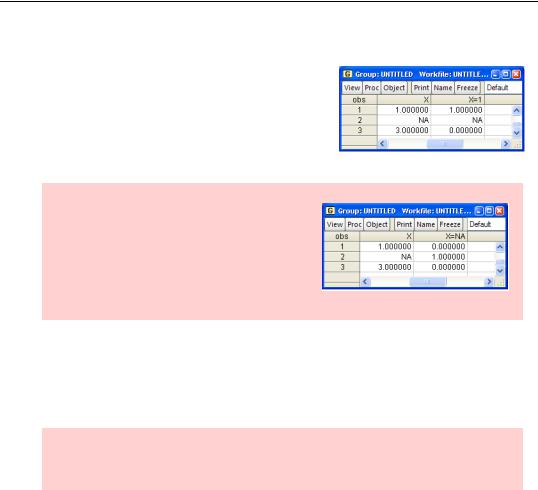
Ordinarily, any operation involving the value NA gives the result NA. Sometimes—particularly in making comparisons—this leads to unanticipated results. For example, you might think the comparison x=1 is true if X equals 1 and false otherwise. Nope. As the example shows, if X is NA then x=1 is not false, it’s NA.
“A foolish consistency is the hobgoblin of little minds” hint: Logically, the result of the comparison x=na should always return NA in line with the rule that any operation involving an NA results in an NA. Logical perhaps, but useless. EViews favors common sense so this operation gives the desired result.
EViews includes a set of special functions to help out with handling NAs, notably @isna(X), @eqna(X,Y), and @nan(X,Y). @isna(X) is true if X is NA and false otherwise. @eqna(X,Y) is true if X equals Y, including NA values. @nan(X,Y) returns X unless X is NA, in which case it returns Y. For example, to recode NAs in X to -999 use X=@nan(X,- 999).
Q: Can I define my own function?
A: No.
Auto-Series and Two Examples
Pretty much any place in EViews that calls for the name of a series, you can enter an expression instead. EViews calls these expressions auto-series.
Showing an expression
For example, to check on our use of @recode on page 91, you can enter an expression directly in a show command, thusly:
show one_2_3 two_3_1 @recode(one_2_3>=two_3_1, one_2_3, two_3_1)
Your Basic Elementary Algebra—93
Auto-series in a regression
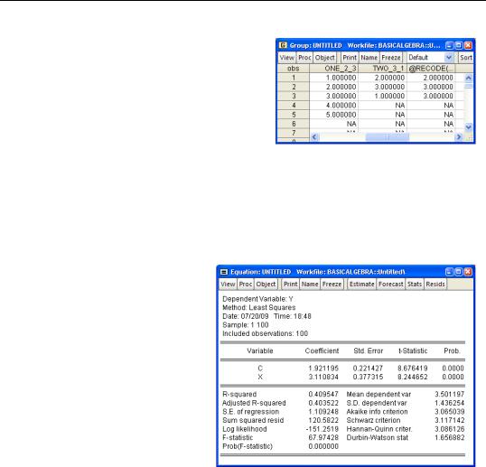
Here’s an example which illustrates the econometric theorem that a regression including a constant is equivalent to the same regression in deviations from means excluding the constant. We can use the random number generators to fabricate some “data”:
rndseed 54321
series x = rnd
series y = 2+3*x + nrnd
Then we can run the usual regression with:
ls y c x
The results are as expected: Both the intercept and slope are close to the values that we used in generating the data.
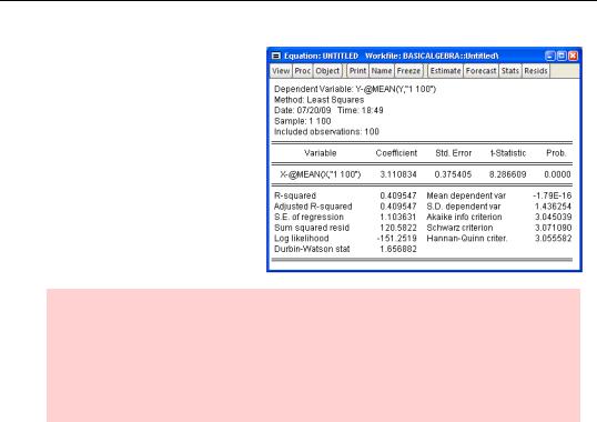
Now we can run the regression in deviations from means and, not incidentally, illustrate the use of auto-series:
ls y-@mean(y) x-@mean(x)
94—Chapter 4. Data—The Transformational Experience
Note that the output from this second regression is identical to the first (demonstrating the theorem but not having anything particular to do with EViews). You’ll also see that EViews has expanded
@mean(y) to @mean(y,
"1 100"). We’ll explain this expansion of the @mean function in just a bit.
Typographic hint: EViews thinks series are separated by spaces. This means that when using an auto-series it’s important that there not be any spaces, unless the auto-series is enclosed in parentheses. In our example, EViews interprets y-@mean(y) as the deviation of Y from its mean, as we intended. If we had left a space before the minus sign, EViews would have thought we wanted Y to be the dependent variable and the first independent variable to be the negative of the mean of Y.
FRML and Named Auto-Series
Have a calculation that needs to be regularly redone as new data comes in, perhaps a calculation you do each month on freshly loaded data? Define a named auto-series for the calculation. When you load the fresh data, the named auto-series automatically reflects the new data.
Named auto-series are a cross between expressions used in a command (y-@mean(y)) and regular series (series yyy = y-@mean(y)). Since it’s simple, we’ll show you how to create a named auto-series and then talk about a couple of places where they’re particularly useful.
Creation of a named auto-series is identical to the creation of an ordinary series, except that you use the command frml rather than series. To create a named auto-series equal to y-@mean(y) give the command:
frml y_less_mean = y-@mean(y)
The auto-series Y_LESS_MEAN is displayed in the workfile window with a variant of the ordinary series icon,  .
.