
- •Table of Contents
- •Foreword
- •Chapter 1. A Quick Walk Through
- •Workfile: The Basic EViews Document
- •Viewing an individual series
- •Looking at different samples
- •Generating a new series
- •Looking at a pair of series together
- •Estimating your first regression in EViews
- •Saving your work
- •Forecasting
- •What’s Ahead
- •Chapter 2. EViews—Meet Data
- •The Structure of Data and the Structure of a Workfile
- •Creating a New Workfile
- •Deconstructing the Workfile
- •Time to Type
- •Identity Noncrisis
- •Dated Series
- •The Import Business
- •Adding Data To An Existing Workfile—Or, Being Rectangular Doesn’t Mean Being Inflexible
- •Among the Missing
- •Quick Review
- •Appendix: Having A Good Time With Your Date
- •Chapter 3. Getting the Most from Least Squares
- •A First Regression
- •The Really Important Regression Results
- •The Pretty Important (But Not So Important As the Last Section’s) Regression Results
- •A Multiple Regression Is Simple Too
- •Hypothesis Testing
- •Representing
- •What’s Left After You’ve Gotten the Most Out of Least Squares
- •Quick Review
- •Chapter 4. Data—The Transformational Experience
- •Your Basic Elementary Algebra
- •Simple Sample Says
- •Data Types Plain and Fancy
- •Numbers and Letters
- •Can We Have A Date?
- •What Are Your Values?
- •Relative Exotica
- •Quick Review
- •Chapter 5. Picture This!
- •A Simple Soup-To-Nuts Graphing Example
- •A Graphic Description of the Creative Process
- •Picture One Series
- •Group Graphics
- •Let’s Look At This From Another Angle
- •To Summarize
- •Categorical Graphs
- •Togetherness of the Second Sort
- •Quick Review and Look Ahead
- •Chapter 6. Intimacy With Graphic Objects
- •To Freeze Or Not To Freeze Redux
- •A Touch of Text
- •Shady Areas and No-Worry Lines
- •Templates for Success
- •Point Me The Way
- •Your Data Another Sorta Way
- •Give A Graph A Fair Break
- •Options, Options, Options
- •Quick Review?
- •Chapter 7. Look At Your Data
- •Sorting Things Out
- •Describing Series—Just The Facts Please
- •Describing Series—Picturing the Distribution
- •Tests On Series
- •Describing Groups—Just the Facts—Putting It Together
- •Chapter 8. Forecasting
- •Just Push the Forecast Button
- •Theory of Forecasting
- •Dynamic Versus Static Forecasting
- •Sample Forecast Samples
- •Facing the Unknown
- •Forecast Evaluation
- •Forecasting Beneath the Surface
- •Quick Review—Forecasting
- •Chapter 9. Page After Page After Page
- •Pages Are Easy To Reach
- •Creating New Pages
- •Renaming, Deleting, and Saving Pages
- •Multi-Page Workfiles—The Most Basic Motivation
- •Multiple Frequencies—Multiple Pages
- •Links—The Live Connection
- •Unlinking
- •Have A Match?
- •Matching When The Identifiers Are Really Different
- •Contracted Data
- •Expanded Data
- •Having Contractions
- •Two Hints and A GotchYa
- •Quick Review
- •Chapter 10. Prelude to Panel and Pool
- •Pooled or Paneled Population
- •Nuances
- •So What Are the Benefits of Using Pools and Panels?
- •Quick (P)review
- •Chapter 11. Panel—What’s My Line?
- •What’s So Nifty About Panel Data?
- •Setting Up Panel Data
- •Panel Estimation
- •Pretty Panel Pictures
- •More Panel Estimation Techniques
- •One Dimensional Two-Dimensional Panels
- •Fixed Effects With and Without the Social Contrivance of Panel Structure
- •Quick Review—Panel
- •Chapter 12. Everyone Into the Pool
- •Getting Your Feet Wet
- •Playing in the Pool—Data
- •Getting Out of the Pool
- •More Pool Estimation
- •Getting Data In and Out of the Pool
- •Quick Review—Pools
- •Chapter 13. Serial Correlation—Friend or Foe?
- •Visual Checks
- •Testing for Serial Correlation
- •More General Patterns of Serial Correlation
- •Correcting for Serial Correlation
- •Forecasting
- •ARMA and ARIMA Models
- •Quick Review
- •Chapter 14. A Taste of Advanced Estimation
- •Weighted Least Squares
- •Heteroskedasticity
- •Nonlinear Least Squares
- •Generalized Method of Moments
- •Limited Dependent Variables
- •ARCH, etc.
- •Maximum Likelihood—Rolling Your Own
- •System Estimation
- •Vector Autoregressions—VAR
- •Quick Review?
- •Chapter 15. Super Models
- •Your First Homework—Bam, Taken Up A Notch!
- •Looking At Model Solutions
- •More Model Information
- •Your Second Homework
- •Simulating VARs
- •Rich Super Models
- •Quick Review
- •Chapter 16. Get With the Program
- •I Want To Do It Over and Over Again
- •You Want To Have An Argument
- •Program Variables
- •Loopy
- •Other Program Controls
- •A Rolling Example
- •Quick Review
- •Appendix: Sample Programs
- •Chapter 17. Odds and Ends
- •How Much Data Can EViews Handle?
- •How Long Does It Take To Compute An Estimate?
- •Freeze!
- •A Comment On Tables
- •Saving Tables and Almost Tables
- •Saving Graphs and Almost Graphs
- •Unsubtle Redirection
- •Objects and Commands
- •Workfile Backups
- •Updates—A Small Thing
- •Updates—A Big Thing
- •Ready To Take A Break?
- •Help!
- •Odd Ending
- •Chapter 18. Optional Ending
- •Required Options
- •Option-al Recommendations
- •More Detailed Options
- •Window Behavior
- •Font Options
- •Frequency Conversion
- •Alpha Truncation
- •Spreadsheet Defaults
- •Workfile Storage Defaults
- •Estimation Defaults
- •File Locations
- •Graphics Defaults
- •Quick Review
- •Index
- •Symbols

78—Chapter 3. Getting the Most from Least Squares
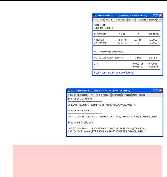
A good example of a hypothesis involving multiple restrictions is the hypothesis that there is no time trend, so the coefficients on both t and t2 equal zero. Here’s the Wald Test view after entering “c(2)=0, c(3)=0”.
The hypothesis is rejected. Note that EViews correctly reports 2 degrees of freedom for the test statistic.
Representing
The Representations view, shown at the right, doesn’t tell you anything you don’t already know, but it provides useful reminders of the command used to generate the regression, the interpretation of the coefficient labels C(1), C(2), etc., and the form of the equation written out with the estimated coefficients.
Hint: Okay, okay. Maybe you didn’t really need the representations view as a reminder. The real value of this view is that you can copy the equation from this view and then paste it into your word processor, or into an EViews batch program, or even into Excel, where with a little judicious editing you can turn the equation into an Excel formula.
What’s Left After You’ve Gotten the Most Out of Least Squares
Our regression equation does a pretty good job of explaining log(volume), but the explanation isn’t perfect. What remains—the difference between the left-hand side variable and the value predicted by the right-hand side—is called the residual. EViews provides several tools to examine and use the residuals.

What’s Left After You’ve Gotten the Most Out of Least Squares—79
Peeking at the Residuals
The View Actual, Fitted, Residual provides several different ways to look at the residuals.
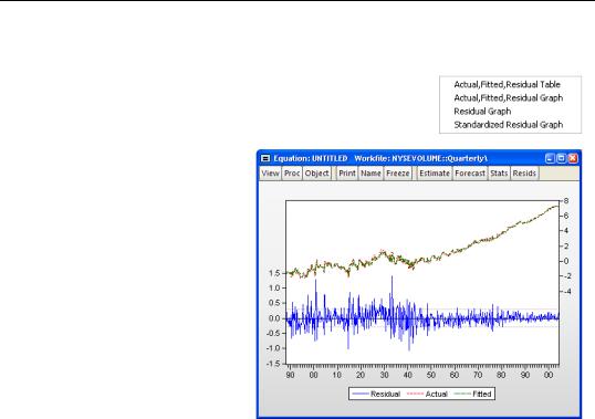
Usually the best view to look at first is Actual, Fitted, Residual/Actual, Fitted, Residual Graph as illustrated by the graph shown here.
Three series are displayed. The residuals are plotted against the left vertical axis and both the actual (log(volume)) and fitted (predicted log(volume)) series are plotted against the vertical axis on the right. As it happens, because our fit is quite good and because we have so many observations, the fitted values nearly cover up the actual val-
ues on the graph. But from the residuals it’s easy to see two facts: our model fits better in the later part of the sample than in the earlier years—the residuals become smaller in absolute value—and there are a very small number of data points for which the fit is really terrible.

80—Chapter 3. Getting the Most from Least Squares
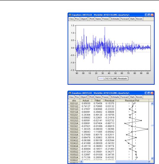
Points with really big positive or negative residuals are called outliers. In the plot to the right we see a small number of spikes which are much, much larger than the typical residual. We can get a close up on the residuals by choosing Actual,
Fitted, Residual/Residual Graph.
It might be interesting to look more carefully at specific numbers. Choose Actual, Fitted,
Residual/Actual, Fitted, Residual Table for a look that includes numerical values.
You can see enormous residuals in the second quarter for 1933. The actual value looks out of line with the surrounding values. Perhaps this was a really unusual quarter on the NYSE, or maybe someone even wrote down the wrong numbers when putting the data together!
Grabbing the Residuals
Since there is one residual for each observation, you might want to put the residuals in a series for later analysis.
Fine. All done.
Without you doing anything, EViews stuffs the residuals into the special series after each estimation. You can use RESID just like any other series.

Quick Review—81
Resid Hint 1: That was a very slight fib. EViews won’t let you include RESID as a series in an estimation command because the act of estimation changes the values stored in RESID.
Resid Hint 2: EViews replaces the values in RESID with new residuals after each estimation. If you want to keep a set, copy them into a new series as in:
series rememberresids = resid
before estimating anything else.
Resid Hint 3: You can store the residuals from an equation in a series with any name you like by using Proc/Make Residual Series… from the equation window.
Quick Review
To estimate a multiple regression, use the ls command followed first by the dependent variable and then by a list of independent variables. An equation window opens with estimated coefficients, information about the uncertainty attached to each estimate, and a set of summary statistics for the regression as a whole. Various other views make it easy to work with the residuals and to test hypotheses about the estimated coefficients.
In later chapters we turn to more advanced uses of least squares. Nonlinear estimation is covered, as are methods of dealing with serial correlation. And, predictably, we’ll spend some time talking about forecasting.

82—Chapter 3. Getting the Most from Least Squares