


A Multiple Regression Is Simple Too—73
tistic” computes the standard F-test of the joint hypothesis that all the coefficients, except the intercept, equal zero. “Prob(F-statistic)” displays the p-value corresponding to the reported F-statistic. In this example, there is essentially no chance at all that the coefficients of the right-hand side variables all equal zero.
Parallel construction notice: The fourth and fifth columns in EViews regression output report the t-statistic and corresponding p-value for the hypothesis that the individual coefficient in the row equals zero. The F-statistic in the summary area is doing exactly the same test for all the coefficients (except the intercept) together.
This example has only one such coefficient, so the t-statistic and the F-statistic test
exactly the same hypothesis. Not coincidentally, the reported p-values are identical and the F- is exactly the square of the t-, 2672 = 51.72 .
Our final summary statistic is the “Durbin-Watson,” the classic test statistic for serial correlation. A Durbin-Watson close to 2.0 is consistent with no serial correlation, while a number closer to 0 means there probably is serial correlation. The “DW,” as the statistic is known, of 0.095 in this example is a very strong indicator of serial correlation.
EViews has extensive facilities both for testing for the presence of serial correlation and for correcting regressions when serial correlation exists. We’ll look at the Durbin-Watson, as well as other tests for serial correlation and correction methods, later in the book. (See Chapter 13, “Serial Correlation—Friend or Foe?”).
A Multiple Regression Is Simple Too
Traditionally, when teaching about regression, the simple regression is introduced first and then “multiple regression” is presented as a more advanced and more complicated technique. A simple regression uses an intercept and one explanatory variable on the right to explain the dependent variable. A multiple regression uses one or more explanatory variables. So a simple regression is just a special case of a multiple regression. In learning about a simple regression in this chapter you’ve learned all there is to know about multiple regression too.
Well, almost. The main addition with a multiple regression is that there are added right hand-side variables and therefore added rows of coefficients, standard errors, etc. The model we’ve used so far explains the log of NYSE volume as a linear function of time. Let’s add two more variables, time-squared and lagged log(volume), hoping that time and timesquared will improve our ability to match the long-run trend and that lagged values of the dependent variable will help out with the short run.
In the last example, we entered the specification in the Equation Estimation dialog. I find it much easier to type the regression command directly into the command pane, although the
74—Chapter 3. Getting the Most from Least Squares
method you use is strictly a matter of taste. The regression command is ls followed by the dependent variable, followed by a list of independent variables (using the special symbol “C” to signal EViews to include an intercept.) In this case, type:
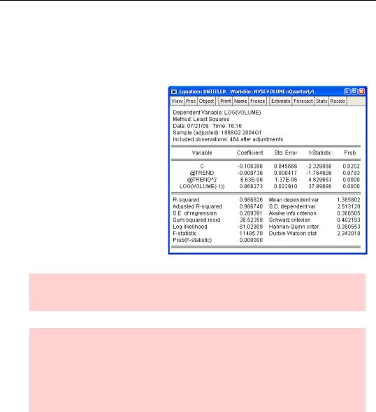
ls log(volume) c @trend @trend^2 log(volume(-1))
and EViews brings up the multiple regression output shown to the right.
You already knew some of the numbers in this regression because they appeared in the second column in Table 1 on page 65. When you specify a multiple regression, EViews gives one row in the output for each independent variable.
Hint: Most regression specifications include an intercept. Be sure to include “C” in the list of independent variables unless you’re sure you don’t want an intercept.
Hint: Did you notice that EViews reports one fewer observation in this regression than in the last, and that EViews changed the first date in the sample from the first to the second quarter of 1888? This is because the first data we can use for lagged volume, from second quarter 1888, is the (non-lagged) volume value from the first quarter. We can’t compute lagged volume in the first quarter because that would require data from the last quarter of 1887, which is before the beginning of our workfile range.
Hypothesis Testing
We’ve already seen how to test that a single coefficient equals zero. Just use the reported t- statistic. For example, the t-statistic for lagged log(volume) is 37.89 with 460 degrees of freedom (464 observations minus 4 estimated coefficients). With EViews it’s nearly as easy to test much more complex hypotheses.
Hypothesis Testing—75
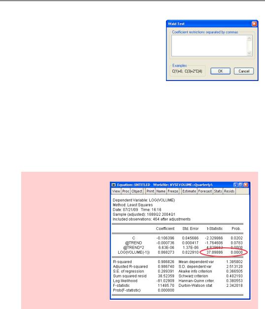
Click the  button and choose Coefficient Diagnostics/Wald – Coefficient Restrictions… to bring up the dialog shown to the right.
In order to whip the Wald Test dialog into shape you need to know three things:
•EViews names coefficients C(1), C(2), C(3), etc., numbering them in the order they appear in the regression. As an example, the coefficient on LOG(VOLUME(-1)) is C(4).
•You specify a hypothesis as an equation restricting the values of the coefficients in the regression. To test that the coefficient on LOG(VOLUME(-1)) equals zero, specify “C(4)=0”.
•If a hypothesis involves multiple restrictions, you enter multiple coefficient equations separated by commas.
Let’s work through some examples, starting with the one we already know the answer to: Is the coefficient on LOG(VOLUME(-1)) significantly different from zero?
Hint: We know the results of this test already, because EViews computed the appropriate test statistic for us in its standard regression output.
76—Chapter 3. Getting the Most from Least Squares
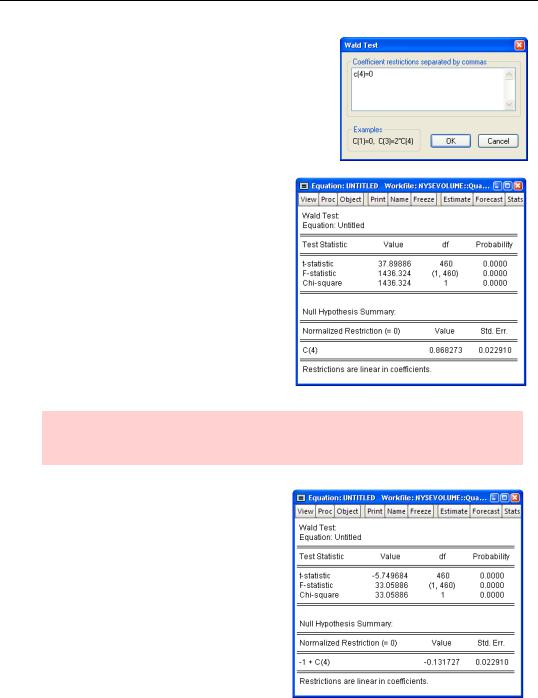
Complete the Wald Test dialog with C(4)=0.
EViews gives the test results as shown to the right.
EViews always reports an F-statistic since the F- applies for both single and multiple restrictions. In cases with a single restriction, EViews will also show the t-statistic.
Hint: The p-value reported by EViews is computed for a two-tailed test. If you’re interested in a one-tailed test, you’ll have to look up the critical value for yourself.
Suppose we wanted to test whether the coefficient on LOG(VOLUME(-1)) equaled one rather than zero. Enter “c(4)=1” to find the new test statistic.
So this hypothesis is also easily rejected.
Hypothesis Testing—77
Econometric theory warning: If you’ve studied the advanced topic in econometric theory called the “unit root problem” you know that standard theory doesn’t apply in this test (although the issue is harmless for this particular set of data). Take this as a reminder that you and EViews are a team, but you’re the brains of the outfit. EViews will obediently do as it’s told. It’s up to you to choose the proper procedure.
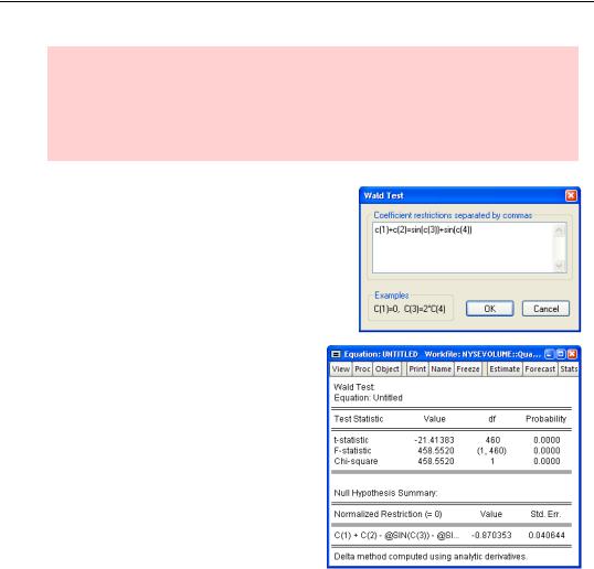
EViews is happy to test a hypothesis involving multiple coefficients and nonlinear restrictions. To test that the sum of the first two coefficients equals the product of the sines of the second two coefficients (and to emphasize that EViews is perfectly happy to test a hypothesis that is complete nonsense) enter “c(1)+c(2)=sin(c(3))+sin(c(4))”.
Not only is the hypothesis nonsense, apparently it’s not true.