66—Chapter 3. Getting the Most from Least Squares

The most important elements of EViews regression output are the estimated regression coefficients and the statistics associated with each coefficient. We begin by linking up the numbers in the inline display—or equivalently column (1) of Table 2—with the EViews output shown earlier.

The names of the independent variables in the regression appear in the first column (labeled “Variable”) in the EViews output, with the estimated regression coefficients appearing one column over to the right (labeled “Coefficient”). In econometrics texts, regression coefficients are commonly denoted with a Greek letter such as a or b or, occasionally, with a Roman b . In contrast, EViews presents you with the variable names; for example, “@TREND” rather than “b ”.

The third EViews column, labeled “Std. Error,” gives the standard error associated with each regression coefficient. In the scientific reporting displays above, we’ve reported the standard error in parentheses directly below the associated coefficient. The standard error is a measure of uncertainty about the true value of the regression coefficient.

The standard error of the regression, abbreviated “ser,” is the estimated standard deviation of the error terms, ut . In the inline display, “ser=0.967362” appears to the right of the regression equation proper. EViews labels the ser as “S.E. of regression,” reporting its value in the left column in the lower summary block.

Note that the third column of EViews regression output reports the standard error of the estimated coefficients while the summary block below reports the standard error of the regression. Don’t confuse the two.

The final statistic in our scientific display is measures the overall fit of the regression line, in the sense of measuring how close the points are to the estimated regression line in the scatter plot. EViews computes R2 as the fraction of the variance of the dependent variable explained by the regression. (See the User’s Guide for the precise definition.) Loosely, means the regression fit the data perfectly and means the regression is no better than guessing the sample mean.

Hint: EViews will report a negative R2 for a model which fits worse than a model consisting only of the sample mean.

The Pretty Important (But Not So Important As the Last Section’s) Regression Results

We’re usually most interested in the regression coefficients and the statistical information provided for each one, so let’s continue along with the middle panel.

68—Chapter 3. Getting the Most from Least Squares

3.Compare the critical value to the t-statistic reported in column four. Find the variable to be “significant” if the t-statistic is greater than the critical value.

EViews lets you turn the process inside out by using the “p-value” reported in the right-most column, under the heading “Prob.” EViews has worked the problem backwards and figured out what size would give you a critical value that would just match the t-statistic reported in column three. So if you are interested in a five percent test, you can reject if and only if the reported p-value is less than 0.05. Since the p-value is zero in our example, we’d reject the hypothesis of no trend at any size you’d like.

Obviously, that last sentence can’t be literally true. EViews only reports p-values to four decimal places because no one ever cares about smaller probabilities. The p-value isn’t literally 0.0000, but it’s close enough for all practical purposes.

Hint: t-statistics and p-values are different ways of looking at the same issue. A t-sta- tistic of 2 corresponds (approximately) to a p-value of 0.05. In the old days you’d make the translation by looking at a “t-table” in the back of a statistics book. EViews just saves you some trouble by giving both t- and p-.

Not-really-about-EViews-digression: Saying a coefficient is “significant” means there is statistical evidence that the coefficient differs from zero. That’s not the same as saying the coefficient is “large” or that the variable is “important.” “Large” and “important” depend on the substantive issue you’re working on, not on statistics. For example, our estimate is that NYSE volume rises about one and one-half percent each quarter.

We’re very sure that the increase differs from zero—a statement about statistical significance, not importance.

Consider two different views about what’s “large.” If you were planning a quarter ahead, it’s hard to imagine that you need to worry about a change as small as one and one-half percent. On the other hand, one and one-half percent per quarter starts to add up over time. The estimated coefficient predicts volume will double each decade, so the estimated increase is certainly large enough to be important for long-run planning.

More Practical Advice On Reporting Results

Now you know the principles of how to read EViews’ output in order to test whether a coefficient equals zero. Let’s be less coy about common practice. When the p-value is under 0.05, econometricians say the variable is “significant” and when it’s above 0.05 they say it’s “insignificant.” (Sometimes a variable with a p-value between 0.10 and 0.05 is said to be “weakly significant” and one with a p-value less than 0.01 is “strongly significant.”) This practice may or may not be wise, but wise or not it’s what most people do.

70—Chapter 3. Getting the Most from Least Squares

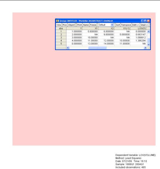
Big (Digression) Hint: Automatic exclusion of NA observations can sometimes have surprising side effects. We’ll use the data abstract at the right as an example.

Data are missing from observation 2 for X1 and from observation 3 for X2. A regression of Y on X1 would use observations 1, 3, 4, and 5. A regression of Y on X2 would use observations 1, 2, 4, and 5. A regression of Y on both X1 and X2 would use observations 1, 4, and 5. Notice that the fifth observation on Y is zero, which is perfectly valid, but that the fifth observation on log(Y) is NA. Since the logarithm of zero is undefined EViews inserts NA whenever it’s asked to take the log of zero. A regression of log(Y) on both X1 and X2 would use only observations 1 and 4.

The variable, X1(-1), giving the previous period’s values of X1, is missing both the first and third observation. The first value of X1(-1) is NA because the data from the observation before observation 1 doesn’t exist. (There is no observation before the first one, eh?) The third observation is NA because it’s the second observation for X1, and that one is NA. So while a regression of Y on X1 would use observations 1, 3, 4, and 5, a regression of Y on X1(-1) would use observations 2, 4, and 5.

Moral: When there’s missing data, changing the variables specified in a regression can also inadvertently change the sample.

What’s the use of the top three lines? It’s nice to know the date and time, but EViews is rather ungainly to use as a wristwatch. More seriously, the top three lines are there so that when you look at the output you can remember what you were doing.

“Dependent Variable” just reminds you what the regression was explaining— LOG(VOLUME) in this case.

“Method” reminds us which statistical procedure produced the output. EViews has dozens of statistical procedures built-in. The default procedure for estimating the parameters of an equation is “least squares.”

72—Chapter 3. Getting the Most from Least Squares

Summary Regression Statistics

The bottom panel of the regression provides 12 summary statistics about the regression. We’ll go over these statistics briefly, but leave technical details to your favorite econometrics text or the User’s Guide.

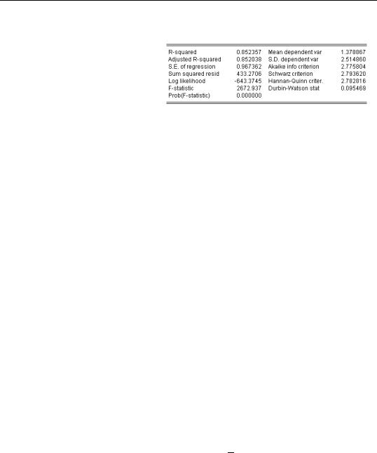
We’ve already talked about the two most important numbers, “R-squared” and “S.E. of regression.” Our regression accounts for 85 percent of the variance in the dependent variable and the estimated standard deviation of the error term is 0.97. Five other elements, “Sum squared residuals,” “Log likelihood,” “Akaike info criterion,” “Schwarz criterion,” and “Hannan-Quinn criter.” are used for making statistical comparisons between two different regressions. This means that they don’t really help us learn anything about the regression we’re working on; rather, these statistics are useful for deciding if one model is better than another. For the record, the sum of squared residuals is used in computing F-tests, the log likelihood is used for computing likelihood ratio tests, and the Akaike and Schwarz criteria are used in Bayesian model comparison.

The next two numbers, “Mean dependent var” and “S.D. dependent var,” report the sample mean and standard deviation of the left hand side variable. These are the same numbers you’d get by asking for descriptive statistics on the left hand side variables, so long as you were using the sample used in the regression. (Remember: EViews will drop observations from the estimation sample if any of the left-hand side or right-hand side variables are NA— i.e., missing.) The standard deviation of the dependent variable is much larger than the standard error of the regression, so our regression has explained most of the variance in log(volume)—which is exactly the story we got from looking at the R-squared.

Why use valuable screen space on numbers you could get elsewhere? Primarily as a safety check. A quick glance at the mean of the dependent variable guards against forgetting that you changed the units of measurement or that the sample used is somehow different from what you were expecting.

“Adjusted R-squared” makes an adjustment to the plain-old R2 to take account of the number of right hand side variables in the regression. R2 measures what fraction of the variation in the left hand side variable is explained by the regression. When you add another right hand side variable to a regression, R2 always rises. (This is a numerical property of least squares.) The adjusted R2 , sometimes written R2 , subtracts a small penalty for each additional variable added.

“F-statistic” and “Prob(F-statistic)” come as a pair and are used to test the hypothesis that none of the explanatory variables actually explain anything. Put more formally, the “F-sta-