

Halilov (ed), Physics of spin in solids.2004
.pdf12 Fulde-Ferrell-Larkin-Ovchinnikov-like state in FM - SC Proximity System
0.6 |
|
|
|
|
|
|
|
2.6 ξS |
|
0.4 |
|
|
|
|
0 |
|
|
|
|
Φ |
|
|
|
|
2πΦ / |
|
|
|
|
0.2 |
9 ξS |
|
|
|
|
15 ξS |
|
|
|
0.0 |
|
|
|
|
0.0 |
0.1 |
0.2 |
0.3 |
0.4 |
|
|
T/Tc |
|
|
Figure 7. The temperature dependence of the total magnetic flux for thickness of the F M slab L/ξS = 2.6 (solid), 6 (dashed) and 15 (dotted curve).
I3 = 4π2tNF4 |
|
e |
|
dω|GF12Nσ(ω)|2 |
|
||||
|
|
|
|
||||||
|
|
|
|
|
|
||||
|
h¯ |
|
σ |
|
|||||
|
|
|
|
|
|
|
|
|
|
ρNNσ11 (ω)ρF22F−σ(ω)[f (ω − eV ) − f (ω)] |
(11) |
||||||||
IA = 4π2tNF4 |
e |
|
|
dω|GF12Fσ(ω)|2 |
|
||||
|
|
|
|
|
|
||||
|
|
|
|
|
|
|
|
||
h¯ |
|
σ |
|
|
|
||||
|
|
|
|
|
|
|
|
||
ρNNσ11 (ω)ρLL22 −σ(ω)[f (ω − eV ) − f (ω + eV )] |
(12) |
||||||||
I1 corresponds to normal electron tunneling between electrodes, I2 is a net transfer of single electron with creation or annihilation of pairs as an intermediate state. I3 corresponds to a process in which electron from normal electron is converted to a hole in superconductor - branch crossing process in language of BT K theroy [35], while IA is the Andreev tunneling.
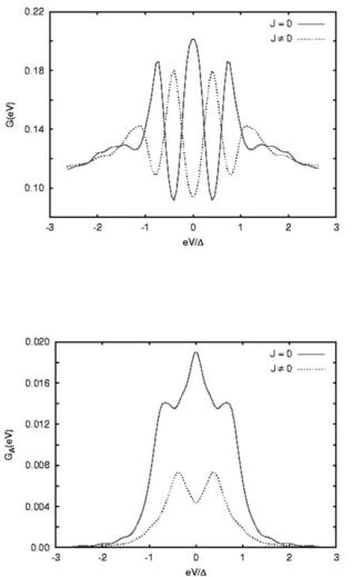
The di erential conductance G(eV ) = dI/d(eV ) as a function of eV = µNM −µSC is shown in the Fig. 8. Clearly, if there is a spontaneous current in the ground state, the conductance peak is split, similarly as in the DOS. We could expect such behavior because G(eV ) is proportional to the DOS at the Fermi energy. And again this e ect could be observable in the tunneling experiments.
We have also extracted Andreev conductance form the total one and ploted in the Fig. 9. We can see that conductance associated with the Andreev processes is strongly enhanced when the current flows in the ground state. Unfortunately it could be very di cult experimentally
Transport properties |
13 |
Figure 8. The total di erential conductance for the solution with and without the spontaneous current.
Figure 9. Corresponding Andreev di erential conductance for the solution with and without the spontaneous current.
measure Andreev conductance only. Despite the fact that for energies less than SC gap the only allowed process is Andreev reflection, as in the point contact geometry, it doesn’t work in our system. The problem is that even at very low energies there is a finite DOS at the Fermi level due to ferromagnet. Naturally the pairing amplitude is induced in F M slab but this is not true energy gap in the quasiparticle spectra and we always deal with some single electron processes in tunneling events.
14 Fulde-Ferrell-Larkin-Ovchinnikov-like state in FM - SC Proximity System
1.62D FFLO state
Before closing discussion on the spontaneous current we wish to make a remark regarding the nature of the ground state in our system. To begin with we recall that recently it has been predicted [36] that under certain conditions a 3D-F F LO state is energetically more favorable than usual 1D state. The 3D state manifests itself in oscillatory behavior of the pairing amplitude not only in the direction perpendicular to the interface but also in direction parallel to it. Moreover, changing the thickness of the F M slab, one can switch the ground state of the system between 3D and 1D-F F LO state [36, 23].
The current carrying ground state of our system can be interpreted as a 2D-F F LO state. The argument is as follows: The oscillations of the pairing amplitude in the direction perpendicular to the interface occur regardless whether the spontaneous current flows or not. Within the F F LO theory [7, 8], the period of the oscillations is related to the x-component of the center of mass momentum of the Cooper pair Q. On the F M side of our model the F F LO periodicity is governed by
Q = (2Eex/vF ) vF , where vF is the Fermi velocity vector. This can be
vF
interpreted as the usual 1D-F F LO state in confined geometry. On the other hand, when the current flows parallel to the interface, there is a finite vector potential in the y-direction. This can be regarded as a y- component of the Q-vector. So one can say that when the spontaneous current flows, the 2D-F F LO state is realized. Moreover when the F M thickness is changed the ground state of the system is switched between 2D- and 1D-state, which manifests itself in spontaneous current flow or in the lack of it. In the present calculations this vector was found during the self-consistency procedure, as it is related to the vector potential in the y-direction. Moreover, the e ective Qy changes its value from layer to layer leading to inhomogeneous F F LO-like state in both dimensions.
1.7Conclusions
The competition between ferromagnetism and superconductivity in F M /SC heterostructures give raise to the Fulde - Ferrell - Larkin - Ovchinnikov (F F LO) state in these systems. The original bulk F F LO state manifests itself in a spatial oscillations of the SC order parameter as well as in spontaneously generated currents flowing in the ground state of the system. We have argued that a very interesting version of this phenomenon accures in F M /SC proximity systems. In short, due to the proximity e ect and Andreev reflections at the F M /SC interface, the Andreev bound states appear in the quasiparticle spectrum. These states can be shifted to the zero energy by tuning the exchange splitting
References |
15 |
or the thickness of the ferromagnet, thus they became zero-energy midgap states which lead to various interesting e ects. In particular, the occurence of spontaneous currents in the ground state can be related to the zero-energy states, as in the case of high-Tc superconductors. It seems that some combination of both phenomena is realized in a real systems. The fact that oscillatory behavior of SC order parameter is strongly correlated with the crossing of the Andreev bound states through Fermi energy and the generation of the spontaneous currents further support F F LO - Andreev bound states picture. The experimental confirmation of the existence of the spontaneous (spin polarized) currents in the ground state would support the F F LO - Andreev bound states scenario in these structures.
Acknowledgments
This work has been partially supported by the grant no. PBZ-MIN- 008/P03/2003.
BLG would like to thank the Center for Computational Material Science (CMS) of TU Wien for hospitality during the preparation of the above talk.
References
[1]C. J. Lambert, R. Raimondi, J. Phys. Condens. Matter 10, 901 (1998).
[2]A. F. Andreev, Sov. Phys. JETP 19, 1228 (1964).
[3]N. F. Berk, J. R. Schrie er, Phys. Rev. Lett. 17, (1966) 433; C. Pfleiderer,M. Uhlarz, S. M. Hayden, R. Vollmer, H. v. Lohneysen, N. R. Bernhoeft, G. G. Lonzarich, Nature 412, (2001) 58; D. Aoki, A. Huxley, E. Ressouche, D. Braithwaite, J. Flouquet, J. -P. Brison, E. Lhotel, C. Paulsen, Nature 413, (2001) 613.
[4]G. E. W. Bauer, Yu. V. Nazarov, D. Huertas-Hernando, A. Brataas, K. Xia, P.
J.Kelly, Materials Sci. Eng. B 84, (2001) 31; S. Oh, D. Youm, M. R. Beasley, Appl. Phys. Lett. 71, (1997) 2376; L. R. Tagirov, Phys. Rev. Lett. 83, (1999) 2058.
[5]G. Blatter, V. B. Geshkenbein, L. B. Io e, Phys. Rev. B 63, (2001) 174511.
[6]M. J. M. de Jong, C. W. J. Beenakker, Phys. Rev. Lett. 74, 1657 (1995).
[7]P. Fulde, A. Ferrell, Phys. Rev. 135, A550 (1964).
[8]A. Larkin, Y. Ovchinnikov, Sov. Phys. JETP 20, 762 (1965).
[9]A. I. Buzdin, L. N. Bulaevskii, S. V. Panyukov, JETP Lett. 35, 178 (1982); A.
I.Buzdin, M. V. Kuprianov, JETP Lett. 52, 487 (1990).
[10]Z. Radovi´c, M. Ledvij, L. Dobrosavljevi´c-Gruji´c, A. I. Buzdin, J. C. Clem, Phys. Rev. B44, 759 (1991).
[11]E. A. Demler, G. B. Arnold, M. R. Beasley, Phys. Rev. B55, 15 174 (1997).
16Fulde-Ferrell-Larkin-Ovchinnikov-like state in FM - SC Proximity System
[12]Y. N. Proshin, M. G. Khusainov, JETP Lett. 66, 562 (1997); M. G. Khusainov,
Y.N. Proshin, Phys. Rev. B56, R14283 (1997); ibid. 62, 6832 (2000).
[13]H. K. Wong, B. Y. Jin, H. Q. Yang, J. B. Ketterson, J. E. Hilliard, J. Low Temp. Phys. 63, 307 (1986).
[14]T. Kontos, M. Aprili, J. Lesueur, X. Grison, Phys. Rev. Lett. 86, 304 (2001).
[15]L. N. Bulaevksii, V. V. Kuzii, A. A. Sobyanin, JETP. Lett. 25, 290 (1977).
[16]M. Sigrist, T. M. Rice, J. Phys. Soc. Japan 61, 4283 (1992).
[17]M. Sigrist, T. M. Rice, Rev. Mod. Phys. 67, 503 (1995); S. Kashiwaya and Y. Tanaka, Rep. Prog. Phys. 63, 1641 (2000); T. L¨ofwander, V. S. Shumeiko, G. Wendin, Supercond. Sci. Technol. 14, R53 (2001).
[18]M. Sigrist, Prog. Theor. Phys. 99, 899 (1998).
[19]P. G. de Gennes and D. Saint-James, Phys. Lett. 4, 151 (1963).
[20]C. Hu, Phys. Rev. Lett. 72, 1526 (1994).
[21]S. V. Kuplevakhskii, I. I. Fal’ko, JETP Lett. 52, 340 (1990).
[22]M. Krawiec, B. L. Gy¨or y, J. F. Annett, Phys. Rev. B66, 172505 (2002).
[23]M. Krawiec, B. L. Gy¨or y, J. F. Annett, European Phys. J. B32, 163 (2003).
[24]M. Krawiec, B. L. Gy¨or y, J. F. Annett, Physica C387, 7 (2003).
[25]K. P. Dunkan, B. L. Gy¨or y, Ann. Phys. (NY) 298, 273 (2002).
[26]M. Fogelstr¨om, S. -K. Yip, Phys. Rev. B57, R14 060 (1998).
[27]S. Higashitani, J. Phys. Soc. Jpn. 66, 2556 (1997).
[28]A. Kadigrobov, R. I. Shekhter, M. Jonson, Z. G. Ivanov, Phys. Rev. B60, 14 593 (1999).
[29]M. Zareyan, W. Belzig, Y. V. Nazarov, Phys. Rev. Lett. 86, 308 (2001).
[30]N. M. Chtchelatchev, W. Belzig, Y. V. Nazarov, C. Bruder, JETP Lett. 74, 323 (2001).
[31]E. Vecino, A. Martin-Rodero, A. L. Yeyati, Phys. Rev. B64 184502 (2001).
[32]M. Krawiec, B. L. Gy¨or y, J. F. Annett, cond-mat/0302162.
[33]L. V. Keldysh, Sov. Phys. JETP 20, 1018 (1965).
[34]J. C. Cuevas, A. Martin-Rodero, A. L. Yeyati, Phys. Rev. B54, 7366 (1996).
[35]G. E. Blonder, M. Tinkham, T. M. Klapwijk, Phys. Rev. B25, 4515 (1982).
[36]Y. A. Izyumov, Y. N. Proshin, M. G. Khusainov, Phys. Usp. 45, (2002) 109; Y.
A.Izyumov, Y. N. Proshin, M. G. Khusainov, JETP Lett. 71, (2000) 138; M.
G.Khusainov, Y. A. Izyumov, Y. N. Proshin, Physica B 284-288, (2000) 503.
EXCHANGE FORCE IMAGE
OF MAGNETIC SURFACES
— A First-Principles Study on NiO(001) Surface —
Hiroyoshi Momida , Tamio Oguchi
ADSM, Hiroshima University
1-3-1 Kagamiyama, Higashihiroshima 739-8530
Japan
Abstract A recently proposed surface atom-probe technique, exchange force microscopy, is examined on an antiferromagnetic NiO (001) surface system. It is shown that atomic force of a ferromagnetic Fe probe on the surface gives a clear spin image when the probe is located within 1˚A above the contact point. Exchange force images show antiferromagnetic pattern of the Ni sites along the [110] direction and asymmetry around the O sites. The asymmetric feature comes from the superexchange interaction between the probe and the second-layer Ni atoms via the surface O ion, being a key proof of the exchange force image on observation.
Keywords: Exchange force microscopy, surface magnetism, first-principles calculation.
2.1Introduction
Exchange force microscopy (EFM) is a spin-dependent extension of non-contact type atomic force microscopy (AFM) by measuring forces acting on a ferromagnetic probe depending on relative spin orientation to the surface atoms [1]. The basic setup of EFM is quite analogous to that of magnetic force microscope (MFM). If the tip and surface are close to each other, typically the order of ˚A, short-range exchange interaction becomes dominant over relatively long-range magnetic dipole one and a spin image of the magnetic surface can be observed in an atomic scale.
present address: National Institute for Materials Science, 1-2-1 Sengen, Tsukuba 305-0047, Japan
17
S. Halilov (ed.), Physics of Spin in Solids: Materials, Methods and Applications, 17–24.C 2004 Kluwer Academic Publishers. Printed in the Netherlands.
18 |
Exchange Force Image of Magnetic Surfaces |
A lot of e orts have been made to development of EFM instrumental setup and surface preparation [2–4] as well as theoretical predictions and quantitative estimation of EFM from first principles [5, 6]. Nakamura has calculated atomic forces between Fe thin films with two kinds of relative magnetization orientations, parallel and anti-parallel, to evaluate exchange force in a realistic system [5]. The magnitude of obtained exchange force is an order of nN, which can be measured with the present non-contact AFM techniques. He found that the exchange force shows an oscillatory behavior as a function of the film distance and that the interaction is dominated by direct exchange between the neighboring d orbitals for short distances while becomes indirect or RKKY-type via more extended s and p orbitals for larger distances. ¿From the lateral variation of the exchange force and its derivative with respect to the distance, it has been concluded that the exchange force may provide us clear information of the spin density distribution of the magnetic surface [6].
However, it may be hard to flip the spin direction of the probe during the observation and more essentially the exchange force cannot be extracted precisely from the atomic force because both atomic and exchange forces have the same symmetry on the ferromagnetic surface. Instead of measuring the ferromagnetic surface with a spin-flipped tip, it should be much easier to measure an anti-ferromagnetic surface with a spin-fixed ferromagnetic tip. This is a quite similar idea to spinpolarized scanning tunneling microscopy (STM) measurement for antiferromagnetic Mn adsorbed on W(110) reported recently [7].
Quite recently we have carried out first-principles calculations for type-II anti-ferromagnetic NiO (001) clean surface to investigate surface structure, electronic structure and spin-density distribution [8]. We have found that the oxygen atoms at the surface may have the spin moment of 0.07µB, which is parallel to that of the Ni atom beneath. In this study, we calculate exchange force of a ferromagnetic Fe probe on antiferromagnetic NiO (001) surface to predict exchange force images of the magnetic surface in an atom scale.
2.2Models and Methods
We calculate atomic forces of a ferromagnetic Fe probe on antiferromagnetic NiO (001) surface to evaluate exchange forces. An important point here is that in case of anti-ferromagnetic surface, we can obtain exchange force with the ferromagnetic tip just by subtracting the forces on antiferromagnetically inequivalent sites. To model such a system, Fe
Results and Discussion |
19 |
mono-layer on 5-layer NiO (001) slab is adopted for the EFM calculations as shown in Fig. 1.
Fe
Ni
Ni 
 Ni
Ni
Ni 
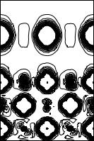
Figure 1. Model system of exchange force microscopy: ferromagnetic Fe monolayer on 5-layer antiferromagnetic NiO(001) slab. Contour plot represents spin density distribution on (100) cross-section. Solid (broken) lines represent positive (negative) spin density. Interval of the density is 0.002 µB /a30, where a0 is the Bohr radius. High spin density region around Ni and Fe is not shown.
For comparison, we have performed electronic structure calculations for clean NiO (001) surface with use of a 9-layer slab model as well as bulk NiO. We use lattice constant of 4.084 ˚A taken from the equilibrium value of bulk NiO. In the present work, we assume no structural relaxation in case of the EFM calculations. We especially focus on probe-height and lateral dependences of the exchange force. The lateral dependence gives us the exchange force images we like to investigate. Our calculations are based on local-spin-density approximation to the density functional theory. One-electron scalar-relativistic Kohn-Sham equations are solved self-consistently by using full-potential linear augmented plane wave (FLAPW) method. The Kohn-Sham wavefunctions are expanded by the basis set with the energy cuto of 15 Ry. The Brillouin zone integration is done by using two-dimensional uniform k-mesh including six k points in the irreducible zone.
2.3Results and Discussion
Electronic Structure and Spin Density in Bulk NiO
Before showing results for NiO surface, let us summarize the electronic structure and spin density in bulk NiO, which have been well studied for a couple of decades. Figure 2(c) shows partial density of states (DOS)
20 |
Exchange Force Image of Magnetic Surfaces |
calculated for bulk antiferromagnetic NiO, which is a reference to the surface system we like to study.
|
3.0 |
(a) Surface |
|
|
|
|
|
|
) |
1.5 |
|
|
|
|
|
|
|
spin |
0.0 |
|
|
|
|
|
|
|
eV atom |
1.5 |
|
|
|
|
|
|
|
3.0 |
(b) Center |
|
|
|
|
|
||
/ |
|
|
|
|
|
|||
|
|
|
|
|
|
|||
( states |
|
|
|
|
|
|
||
1.5 |
|
|
|
|
|
|
|
|
0.0 |
|
|
|
|
|
|
|
|
OF STATES |
|
|
|
|
|
|
|
|
1.5 |
|
|
|
|
|
|
|
|
3.0 |
(c) Bulk |
|
|
|
|
|
||
DENSITY |
1.5 |
|
|
|
|
|
|
|
0.0 |
|
|
|
|
|
|
|
|
1.5 |
|
|
|
|
|
|
|
|
|
|
|
|
|
|
|
|
|
|
3.0 |
|
-8 |
-6 |
-4 |
-2 |
0 |
2 |
|
-10 |
|||||||
ENERGY ( eV )
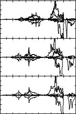
Figure 2. Calculated partial density of states of (a) surface layer and (b) center layer in 9-layer NiO(001) slab and (c) bulk NiO. Thick solid, thin solid and broken lines denote O-p and Ni-d eg and t2g components, respectively. The energy zero is taken at the top of the valence band of each system. Top and bottom panels represent the majority and minority spin states, respectively, of each layer.
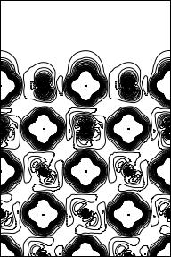
Spin magnetic moment at the Ni site is 1.16µB, which comes from hole in Ni-d eg (3z2 − r2 and x2 − y2) minority-spin band. So, the spindensity distribution around Ni reflects the shape of the eg orbital, as equivalently shown in the spin density distribution in the center layer of the NiO slab in Fig. 3.
There is strong hybridization between O-p and Ni-d eg orbitals and certain hole amplitude may exist also at the O sites. One can see weak spin-density distribution around O in Fig. 3 but its integrated quantity, namely spin moment, becomes zero at the O sites by symmetry.
Electronic Structure and Spin Density in NiO (001)
Surface
Contrast to the bulk NiO, the O ions may have finite size of spin moment at surface because of symmetry breaking. Actually we get such finite spin moment at surface O sites as much as 0.07µB. The surface spin moment is parallel to that of the Ni site underneath and originates in O-pz orbital as shown in Fig. 3. The O spin moments are diminished
Results and Discussion |
21 |
Ni
Ni |
Ni |
Ni
Ni |
Ni |
Figure 3. Calculated spin density distribution on (100) cross-section in 9-layer NiO (001) slab. Solid (broken) lines represent positive (negative) spin density. Interval of the density is 0.002 µB /a30, where a0 is the Bohr radius. High spin density region around Ni is not shown.
quickly beyond the second layer, approaching to the bulk value. On the other hand, the spin density distribution around Ni and the spin moments are very rigid in nature.
Figure 2 shows partial DOS of the surface and center layer. Calculate DOS of the center layer is just like bulk DOS while one can see a reduction of the band gap at surface due to Ni-d eg orbital. This reduction comes from lack of hybridization of the eg orbital vertical to the surface (3z2 − r2 component) while surface-parallel (x2 − y2) component of the eg orbital is still bulk-like. Small spin polarization at the O sites can be recognized, mostly originating from O-pz orbital.
Atomic and Exchange Forces of Fe Probe on NiO(001) Surface
Calculated atomic forces are smooth functions of the probe height as shown in Fig. 4.
The probe height is taken as the distance between the Fe mono-layer and the surface layer of NiO (001) (see Fig. 1). The Fe probe atoms are attracted more strongly by O than by Ni. But exchange force, which is defined as the atomic force di erence between di erent spin orientations