

Rivero L.Encyclopedia of database technologies and applications.2006
.pdfMathematics of Generic Specifications for Model Management, II
presentation of this instance is shown on the left.
For interpreting items of the relational metaschema, sketch Mske must be augmented with the corresponding derived items. They are shown by dashed gray (green on a color display) lines and defined as specified by Figure 1A; their names are prefixed with slash, as suggested by UML. Now we can explicate correspondence between sketch and relational schemas by building an interpreta-
tion mapping m: Mrel→ derQMske. This mapping is specified in Figure 1 by labeling the Mrel’s items by Mske’s items; labels stand after colon in Mrel-items’ names and are
shown in violet on a color display.
DATA TRANSLATION IS DETERMINED BY METAMODEL INTERPRETATION
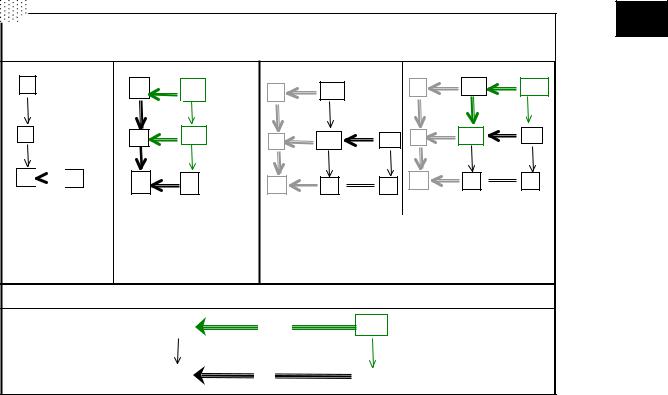
We will see how metamodel interpretation governs the entire transformation procedure. To illustrate the idea, we apply the general procedure to a very simple piece of data shown in the left-most upper cell of Figure 1.
The first step is to present data as a graph mapping δ: D → S from the data graph to the schema graph, and the schema (data on the metalevel) as a graph mapping σ: S → M into the metaschema graph. These mappings, specified via labeling (as described above), are shown in the left column half of Figure 1 (by the abuse of notation, we use labels of schema arrows as their “names” for labeling the data-graph arrows). Identifiers for the four data links in the leftmost top cell are denoted in graph D by #P_i, i=1,..,4).
Definitions of derived items augmenting the metaschema are query specifications for its instances— schemas. Executing these queries augments the schema with derived items shown in the dashed lines, which, in their turn, are query specifications for data and propagate to augmenting data. In this way we obtain a chain of
extended mappings D →δ S →σ M = Mske , where overlined capital letters denote augmented graphs. To simplify notation, further in the article we will always interpret arrows by Kleisly mappings and omit bars over objects’ and arrows’ names. In other words, we will work in a Kleisly category over graphs (determined by a choice of legitimate operations/queries with data; see Math-I).
The next step is to select that part of the schema sketch S, which is mapped by σ into the range of the interpretation m, and rearrange its labeling to sketch Mrel. This is
σ m
done by applying to the span S →Mske ← Mrel the diagram operation of meet explained in Table 2 of Math- I. The result is a new graph /S* together with two mappings:
vertical, /σ*: /S* → Mrel, and horizontal, S ←/ m* / S *.3
The vertical mapping is shown in the right middle cell of Figure 1; it makes /S* a relational schema. The horizontal mapping (informally described by the visual graphic similarity between /S* and S) relates /S* with the original schema sketch and shows how the labels are changed.
Finally, we select that part of the data graph D, which is mapped by δ into the range of the schema mapping /m*, and rearrange its labeling to graph /S*. This is again done by applying the meet-operation and produces a new graph /D* together with two mappings:
vertical, /δ*: /D* → /S*, and horizontal, ** .
D←/ m / D*
The former mapping makes data graph /D* an instance over schema /S*, and the latter relates it to the original data graph.
Properties of the interpretation m determine properties of the entire procedure. Since in our example m is injective (one-one) and the meet-operation preserves injectivity, objects /S* and /D* are, in fact, sub-objects of their sketch-format counterparts. In fact, we did nothing but select these sub-objects and rearrange their labeling. Thus, for one-one mapping m, meet works with labels of data items rather than with data itself.
Another special property of our example is that the schema sketch S is so simple that the range of mapping σ comes to be inside of the range of mapping m, i.e., inside
of the image of Mrelunder m. Hence, no data item was lost during the transformation. In general, the full sketch
format is richer than relational, and some part of the full sketch metamodel goes beyond the range of m. If a piece of data, D, has a schema whose image under mapping σ goes beyond the range of m, then some data items from D will be lost during the transformation.
Considering this simple example in abstract terms leads to a generic pattern of data and schema transformation. It is described in the next section.
DATA TRANSFORMATION VIA DIAGRAM CHASING
Table 1 presents an abstract generic specification of data transformation in the general setting described at the beginning of the article. The input information for the entire procedure is formed by (1) a data instance D1 over a source schema S1 and (2) two Kleisly morphisms: metaschema interpretation m12: M2ѲM1 and schema mapping (view) s12: S2 Ѳ/S1* of the target schema into the M2 translation of the source schema. All the rest is done automatically by consecutive application of the two ge-
360
TEAM LinG
Mathematics of Generic Specifications for Model Management, II
Table 1. Generic format of data transformation
|
Heterogeneous MMt |
|
Homogeneous MMt |
||
|
|
|
|
|
|
Step 1 |
|
Step 2 |
Step 3 |
|
Step 4 |
|
|
|
|
||
D1
δ1
S1
σ1
M1 

 M2
M2
m12
Specifiyng 1st half of input data for the operation: metaschema interpretation (Kleisly arrow) m12
D1 |
/m12** |
/D1* |
|
/m12** |
|
|
|
|
/m12** |
/D1* |
/s12* |
/D1** |
D1 |
/D1* |
|
|
D1 |
|
|
||||||
δ1 |
[meet] |
/δ1* |
δ1 |
[meet] /δ1* |
|
|
δ1 |
[meet] /δ1* |
[meet] /δ1** |
|||
S |
/m12* |
/S1* |
S1 |
/m12* |
* |
|
S2 |
S |
/m12* |
/S1* |
|
S2 |
1 |
|
|
|
/S1 |
s12 |
1 |
|
|
s12 |
|
||
σ1 |
[meet] |
/σ1* |
|
|
|
|
σ1 |
[meet] |
/σ1* |
σ2 |
||
σ1 |
[meet] |
/σ1* |
σ2 |
|
||||||||
M1 |
|
M2 |
M1 |
|
M2 |
|
M2 |
M1 |
m12 |
M2 |
id |
M2 |
|
m12 |
|
|
id |
|
|
|
|||||
|
|
|
m12 |
|
|
|
|
|
||||
|
|
|
|
|
|
|
|
|
|
|||
Translating schema S1 into |
Entering 2nd half of input |
Rearranging data /D1* into data |
schema /S1* in metamodel M2 |
data for the operat i on: |
/D1** over schema S2. |
and then rearranging the data |
schema S2 in metamodel M2 |
|
D1 to data /D1* over schema |
together with a view (Kleisly |
|
/S1* |
arrow) s12 to schema /S1* |
|
|
|
|
Quasi-homogeneous MMt: Overall specification of Steps 1…4 via Grothendick arrows and operations with them
|
|
/s12* |
/D1** |
|
|
D1 |
|||
δ1 |
[[meet]] |
** |
||
|
||||
|
|
|
/ δ1 |
|
|
|
s12 |
|
|
|
S1 |
S2 |
|
|
|
|
|
||
M
neric diagram operations: Kleisly expansion for vertical arrows (see section “Kleisly Operation” in Math-I) and meet for the left-lower arrow spans (Table 2 in Math-I).
In more detail, after we have translated data and schema over metamodel M1 into metamodel M2 (see Steps 1 and 2 in Table 1), we can safely specify the target schema S2 as a view to the schema /S1*, that is, as a (homogeneous) Kleisly mapping s12: S2Ѳ/S*1 (Step 3 in Table 1). Computing data D2 is now nothing but computing a (materialized) view of data D1 specified by schema S2. This computation is performed by applying the diagram operation meet once again (Step 4).
Note, the metaschema interpretation m12 sets the base of the entire procedure and in much determines its properties. Strictly speaking, we cannot even talk about schema S2 as a view to schema S1 until S1 is translated to a form similar to S2 (to S2 metaschema’s terms). On the other hand, we can introduce a new sort of arrows between schemas, say, f: S T, which would be a shorthand for pairs (m,s) with m: MS ѲMT, a Kleisly arrow (itself a shorthand!) between metaschemas and s: S → /T*, a homogeneous schema mapping. The target of this mapping, /T*, is the translation of schema T into the MS terms according to interpretation m as described above. We will call such arrows Grothendieck morphisms or mappings, after Alexander Grothendieck, the inventor of this fundamental categorical construct.
Grothendieck mappings provide a very convenient abbreviation. With Grothendieck arrows we can specify heterogeneous MMt procedures as if we are living in a homogeneous model world. For example, the task of data transformation looks like a simple view computation; see the lower half of Table 1. For another example, heterogeneous model merge can be specified as shown in the right-most column of Table 1 in Math-I but with Kleisly arrows replaced by Grothendieck arrows. Implementation, however, needs de-abbreviating the Grothendieck arrows and operations with them into arrows between model representations and operations over them, as shown in the upper half of Table 1 here.
CATEGORICAL FOUNDATIONS FOR
GENERIC MMt SPECIFICATIONS
Consider specifications in Table 1 of Math-I and Table 1 in this article once again. We have directed graphs, whose nodes denote data and schema representations, and arrows are mappings between them. The graphs are endowed with marked diagrams denoting either operations with representations and their mappings, for example, [meet] and [join], or properties of their configurations, for example, in cell (b) of Table 1 in Math-I, the pair of arrows /f1Σ, /f2Σ is declared to be covering as specified by the marker [cover]. Another example of a diagram
361
TEAM LinG

Mathematics of Generic Specifications for Model Management, II
Table 2. Abstract MMt in categorical light
|
Elementary Units |
Repository |
Elementary Query |
A Complete Query Language |
|
|
|
Structure |
|
|
|
Data |
Value |
Set of relations |
Relational |
Relational algebra (a version of |
|
first-order predicate calculus) |
|||||
|
(tables) |
operation |
|||
Management |
|
||||
|
|
||||
|
|
|
|
||
Model |
Model, mapping |
Sketch of models |
Diagram operation |
MMt doctrine/topos |
|
Management |
|
and mappings |
(a version of higher-order |
||
|
|
||||
|
|
|
|
intuitionistic predicate calculus) |
property is commutativity of all arrow squares involved (by default). Thus, our meta-specifications are sketches in some signature of diagram operations and predicates.
This format is generic across metamodels simply because metamodels are included into specifications, either explicitly, as in the upper part of Table 1, or implicitly, when we interpret arrows by Grothendieck mappings. The format is also generic across applications: Other MMt tasks may require other diagram operations and predicates to be applied, but the very pattern remains the same. Since operations involved should inevitably include arrow composition, the sketches we discuss are finite presentations of categories endowed with an extra structure.
This extra structure consists of two components. The first is a Kleisly structure, Q. It is formed by query operations of augmenting nodes (representations) with new items and the corresponding expansions of arrows (see section “Model Mappings as Kleisly Arrorws” in Math-I). The second component is an algebra A of diagram operations (over representations and their mappings as holistic entities); see Table 2 in Math-I for examples. Using the notion of Kleisly mapping, we can “hide” the structure Q inside of the arrows and consider diagram operations over the Kleisly category R[Q]. Thus, the MMt universe can be considered as a pair (R[Q], A) with R[Q] a category of model representations and Kleisly mappings between them, and A a diagram algebra over it.
A question of fundamental importance for gMMt is whether there exists a set of diagram operations whose compositions can generate any MMt operation of practical interest (of course, here we do not consider heuristic MMt operations like schema matching). This sort of problem was studied in Category Theory in detail, and roughly the results are as follows.
Endowing a category C with a certain set of diagram operations A allows interpreting logical calculi in C, and the other way round, a pair (C, A) generates a certain logical calculus (the so-called internal language of C). In this way a category endowed with an extra algebraic structure and a logical calculus turn out to be basically equivalent constructs.4 That is why pairs (C,A) are called (logical) doctrines in categorical logic.
An important aspect of the notion of doctrine is that
the component A actually refers to the entire pool of diagram operations legitimate over C rather than to a specific set of basic operations generating A by composition. Such pools of operations closed under composition are sometimes called clones. Thus, the notion of doctrine refers to a clone of diagram operations rather than to a specific set of operations generating it.5
A fine hierarchy of doctrines and their calculus counterparts was built in Category Theory. In the top part of the hierarchy are algebraically and logically rich categories called toposes, whose logical calculus counterparts are higher-order predicate logics, type theories, and constructive set theories. Roughly, in a topos one can perform all constructive operations with objects which one would normally enjoy with ordinary sets; particularly, take intersections and unions of objects, form their images and co-images under given morphisms, consider graphs (binary relations) of morphisms, take transitive closures of binary relations, and much more. Surprisingly, this extremely rich pool of manipulations with objects is generated by compositions of only three basic diagram operations: arrow composition, meet, and powerset (building the object of all sub-objects of a given object).
The category of graphs is proven to be a topos, and hence, every constructive operation with graphs can be presented as a composition of three basic topos operations. However, the powerset operation is extremely noneffective and, hence, should be excluded from the clone of MMt operations AMMt. Thus, the latter is a proper sub-
clone of the clone of topos operations ATop, AMMt ATop. Since powerset is excluded from AMMt, we face the problem
of finding an appropriate set of basic operations generating the entire clone AMMt. This set should include image, meet, join (see Table 2 in Math-I), some restricted version of powerset (discussed in Diskin & Kadish, 2003), and, perhaps, a few other important operations, which could be derived (in a topos) with the powerset operation but without it must be included into the basic set. Finding the latter is currently an open question. Nevertheless, there
should be an object (CMMt., AMMt.) in the hierarchy of doctrines—let us call it MMt doctrine or MMt topos—in
which algebra A consists of effective diagram operations covering all gMMt’s needs.6
362
TEAM LinG
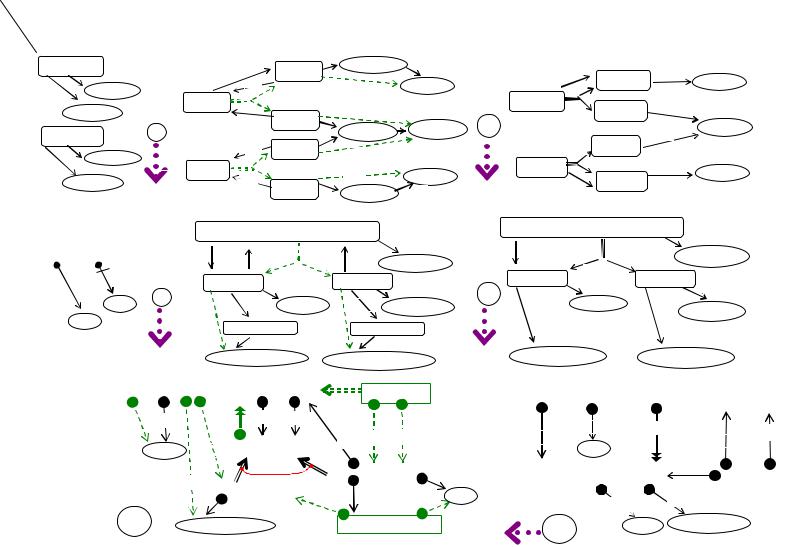
Figure 1. Example of data translation: sketches into relational tables
|
|
|
|
|
|
|
|
|
|
|
Sketch data model |
|
|
|
|
|
|
|
|
|
|
|
|
|
|
|
|
|
|
|
|
|
|
|
|
|
|
|
|
|
|
|
Relational data model |
|
|
|
|
|
|
|
|
||||||||||||||||||||
|
|
|
|
Visual |
|
|
|
|
|
|
|
|
|
|
|
|
|
|
|
|
|
|
|
|
|
|
|
Data and Schemas as Graph Mappings |
|
|
|
|
|
|
|
|
|
|
|
|
|
|
Visual |
|
|
|
|||||||||||||||||||||||||
|
|
|
|
Presentation |
|
|
|
|
|
|
|
|
|
|
|
|
|
|
|
|
::ta |
|
|
|
|
|
|
|
|
|
|
|
|
|
|
|
|
|
|
|
|
|
|
|
|
|
|
|
|
|
|
|
|
|
|
|
|
|
Presentation |
|
|||||||||||
|
|
|
#O1 :Person |
|
|
|
|
|
|
|
|
|
|
|
|
|
|
|
|
|
|
“002” :#N2 |
|
:type |
|
|
|
|
|
|
|
|
|
|
|
|
|
|
|
|
|
|
|
|
|
|
|
|
|
|
|
|
|||||||||||||||||||
|
of |
|
|
|
|
|
|
|
|
::key |
|
|
|
#P1 :#A1 |
|
|
|
|
|
|
|
|
|
|
::p-key |
|
|
#P1* :#A1* |
::dom |
|
|
|
|
|
|
|
|
||||||||||||||||||||||||||||||||||
|
|
|
:pin |
|
|
|
|
|
|
|
|
|
|
|
|
|
|
|
|
|
|
|
|
|
|
|
|
|
|
|
|
|
|
|
|
|
|
|
|
|
|
|
|
|
|
|
|
|
|||||||||||||||||||||||
|
, D, is aninstance |
|
|
|
|
|
|
|
|
|
|
|
|
::so |
|
|
|
|
|
|
|
|
|
|
|
|
|
|
|
|
|
|
|
|
|
|
|
|
|
|
|
|
|
|
|
|
|
|
|
|
|
|
|
|
|
|
|
|
|
||||||||||||
|
|
|
:name |
“002” :int |
|
|
|
|
|
|
|
|
|
|
|
|
|
|
|
|
|
::dom |
|
|
|
|
|
“002” :int |
|
|
|
|
|
|
|
|
|
|
|
|
|
|
|
|
“002” :int |
|
|
|
|
|
|
|
|
||||||||||||||||||
|
|
|
|
|
|
|
|
|
|
|
|
|
|
|
|
|
|
|
|
|
|
|
|
|
|
|
|
#O1* :#N1* |
|
|
|
|
|
|
|
|
|
|
|
|
|
|
|
|
|
|
|
|
|||||||||||||||||||||||
|
the schema S |
|
|
|
|
#O1 :#N1 |
|
::/out |
|
|
|
|
|
|
|
|
|
|
|
|
|
|
|
|
|
|
|
|
|
|
|
|
|
|
|
|
|
|
|
|
|
|
|
|
|
|
|
|
|
|
|
|
|||||||||||||||||||
|
|
“Lee” :str |
|
|
|
|
|
|
|
|
|
|
|
::dom |
|
|
|
|
|
|
|
|
|
|
|
|
|
|
|
#P2* :#A2* |
::dom |
|
|
|
|
|
|
|
|
||||||||||||||||||||||||||||||||
|
|
|
|
|
|
|
|
|
|
|
|
|
#P2 :#A2 |
|
|
|
|
|
|
|
|
|
|
|
|
|
|
|
|
|
|
::clmn-list |
|
|
PERSON |
|
|||||||||||||||||||||||||||||||||||
|
|
|
|
|
|
|
|
|
|
::so |
|
|
|
|
|
|
|
|
|
|
|
|
|
|
|
|
|
|
|
|
|
|
|
|
|
|
|
|
|
|
|
|
|
|
|
|
|
||||||||||||||||||||||||
|
|
|
|
|
|
|
|
|
|
|
|
|
|
|
|
|
|
|
|
|
|
|
“Lee” :str |
/D* |
|
|
|
|
|
|
|
|
|
|
|
|
“Lee” :str |
|
|
|
|||||||||||||||||||||||||||||||
|
|
#O2 :Person |
|
|
|
|
|
|
|
|
|
|
|
|
|
::ta |
|
|
|
“Lee” :#N3 |
|
|
|
|
|
|
|
|
|
|
|
|
|
|
|
|
|
|
|
|
|
|
|
|
|
|
|
||||||||||||||||||||||||
|
|
|
|
D |
|
|
|
|
|
|
|
|
|
|
|
|
|
|
|
|
|
|
|
|
|
|
|
|
|
|
|
|
|
::dom |
|
|
pin |
|
|
name |
|
||||||||||||||||||||||||||||||
|
|
|
|
|
|
|
|
|
|
|
|
|
|
|
#P4 :#A2 |
|
|
|
|
|
|
|
|
|
|
|
|
|
|
|
|
|
|
/δ * |
|
|
|
|
|
::clmn-list #P4*:#A2* |
|
|
|
|
|
|
|
|
|
|
|
|
|
|
|||||||||||||||||
|
|
|
|
|
|
|
|
|
|
|
|
|
::so |
|
|
|
|
|
|
|
|
|
|
|
|
|
|
|
|
|
|
|
|
|
|
|
|
|
|
|
002 |
|
|
Lee |
|
||||||||||||||||||||||||||
|
|
:pin |
|
|
|
|
|
|
|
|
|
|
|
|
::dom |
|
|
|
|
|
|
|
|
|
|
|
|
|
|
|
|
|
|
|
|
|
|
|
|
|
|
|
|
||||||||||||||||||||||||||||
|
“005” |
:int |
|
δ |
|
|
|
|
|
|
|
|
|
|
|
|
|
|
|
|
|
|
|
|
|
|
|
|
|
|
|
|
|
|
|
|
|
|
|
|
|
|
|
|
|
|
|
|
::dom |
|
|
|
|
|
|
||||||||||||||||
|
:name |
|
|
#O2 :#N1 |
::/out |
|
|
|
|
|
|
|
|
|
|
|
|
|
|
|
|
|
|
|
|
|
|
|
|
#O2* :#N1* |
|
|
|
|
|
|
005 |
|
|
Lee |
|
||||||||||||||||||||||||||||||
|
|
|
|
|
|
|
|
|
|
|
|
|
|
::dom |
|
|
|
|
|
|
|
|
|
|
|
|
|
|
|
|
|
|
|
|
|
|
“005” :int |
|
|
|
|
||||||||||||||||||||||||||||||
|
Data |
|
|
|
|
|
|
|
|
|
|
|
|
|
|
|
|
|
|
|
|
“005” :int |
|
|
|
#P3* :#A1* |
|
|
|
|
|
|
|
|
|
||||||||||||||||||||||||||||||||||||
|
|
|
|
|
|
|
|
|
|
|
|
|
|
|
|
|
|
|
|
|
|
|
|
|
|
|
|
|
|
|
|
|
|
|
|
|
|
|
|
|
|
||||||||||||||||||||||||||||||
|
|
|
“Lee” :str |
|
|
|
|
|
|
|
|
::so |
#P3 :#A1 ::ta |
|
|
|
|
|
|
|
|
|
|
|
|
|
|
|
|
|
|
|
|
|
|
|
|
|
|
|
|
|
|||||||||||||||||||||||||||||
|
|
|
|
|
|
|
|
|
|
|
|
|
|
|
|
|
|
|
|
|
|
/S* |
|
|
|
|
|
::p-key |
|
|
|
|
|
|
|
|
|
|
|
|
|
|
|||||||||||||||||||||||||||||
|
|
|
|
|
S |
|
|
|
|
|
|
“005” :int |
|
|
::type |
|
|
|
|
|
|
|
|
|
|
|
|
|
|
|
|
|
|
|
|
|
|
|
|
|
|
|
|
||||||||||||||||||||||||||||
|
|
|
|
|
|
|
|
|
|
|
|
|
|
|
|
|
|
|
|
|
|
|
|
|
|
|
|
|
|
|
|
|
|
|
|
|
|
|
|
|
|
|
|||||||||||||||||||||||||||||
|
|
|
|
|
|
|
|
|
|
|
|
|
|
|
|
|
|
|
|
|
|
|
|
|
|
|
|
|
|
|
|
|
|
|
|
|
|
|
|
|
|
|
|
|
|
|
|
|
|
|
|
|
|
|
|
|
|
|
|
|
|
|
|
|
|
|
|
|
|
|
|
|
of |
|
|
|
|
|
|
|
|
|
|
|
|
|
#N1 :objectClass |
|
|
|
|
|
|
|
|
|
|
|
|
|
|
|
|
|
|
|
|
|
|
|
|
#N1* :Table |
|
|
|
|
:name |
|
|
|
|
|
|
|
|
||||||||||||||||||
|
S, isan instance |
|
|
|
|
|
|
|
|
|
|
|
:key |
|
|
|
|
|
|
|
|
|
|
|
|
|
|
|
|
|
|
|
|
:name |
|
|
|
|
|
|
|
|
|
|
|
|
|
|
:clmn-list |
|
|
|
Table PERSON ( |
|
|||||||||||||||||
|
metamodel M |
|
Person |
|
|
|
|
|
|
|
:so |
|
|
|
|
:/out |
|
|
|
|
|
|
|
|
|
|
|
|
|
|
|
|
|
|
|
|
:p-key |
|
|
|
|
|
|
|
“Person” :str |
|
|
||||||||||||||||||||||||
|
|
|
|
|
|
|
|
|
|
|
|
|
|
|
|
|
|
|
|
|
|
|
|
|
|
|
|
|
|
|
|
|
|
|
|
|
|
|
|
|
|
|
|
|
|
|
|||||||||||||||||||||||||
|
|
|
|
|
|
|
|
|
|
|
|
|
|
|
|
|
|
|
|
|
|
:so |
|
|
“Person” :str |
|
|
|
|
|
|
|
|
: 1 |
: 2 |
|
|
|
|
pin int |
p-key |
|
|||||||||||||||||||||||||||||
|
|
|
|
|
|
|
|
|
|
|
|
|
|
|
|
|
|
|
|
|
|
|
|
|
|
|
|
|
|
|
|
|
|
|
|
|
|
|
|
|
|
|
|
|
|
||||||||||||||||||||||||||
|
|
|
|
|
|
|
|
|
|
|
|
|
|
|
|
: 1 |
|
|
: 2 |
|
|
|
|
|
|
|
|
|
|
|
|
|
|
|
|
|
|
|
|
|
|
|
|
|
|
|
|
|
|||||||||||||||||||||||
|
|
|
|
[key] |
|
|
|
|
#A1 :Arrow |
|
|
|
|
|
|
#A2 :Arrow |
|
|
|
|
|
|
|
|
|
|
|
#A1* :Clmn |
|
#A2* :Clmn |
|
|
|
|
|
name |
str |
|
|
|
|||||||||||||||||||||||||||||||
|
|
|
pin |
|
|
|
|
|
|
|
|
|
|
|
|
|
|
|
|
|
|
|
|
|
|
|
|
|
|
|
|
|
|
|
|
|
|
||||||||||||||||||||||||||||||||||
|
|
|
|
|
|
|
:name |
|
|
|
:name |
|
|
|
|
|
|
|
|
|
|
|
|
|
|
||||||||||||||||||||||||||||||||||||||||||||||
|
|
|
|
|
|
|
|
|
|
|
|
|
|
|
|
|
|
|
:name |
|
|
|
|
|
|
|
|
||||||||||||||||||||||||||||||||||||||||||||
|
|
name |
|
|
|
S |
|
|
|
|
|
|
|
|
|
|
|
|
|
|
|
|
|
|
|
|
/S* |
|
|
|
|
|
:name |
|
|
|
|
|
|
|
|
|
|
); |
|
|
|
|
|
||||||||||||||||||||||
|
|
[int] |
|
|
|
|
|
|
|
|
|
|
|
|
|
|
|
|
|
|
|
|
|
|
|
|
|
|
|
|
|
|
|
|
|
|
|
|
|
|
“pin" :str |
|
|
|
|
|
|
|
|
|
|
|
|
|
|||||||||||||||||
|
|
|
|
σ |
|
:/dom |
:ta |
|
|
“pin" :str |
|
|
|
|
:ta |
|
|
“name” :str |
/σ* |
|
|
|
:dom |
:dom |
|
|
“name” :str |
|
|
|
|
|
|
|
|
||||||||||||||||||||||||||||||||||||
|
|
|
|
|
|
|
|
|
|
|
|
|
|
|
|
|
|
|
|
|
|
|
|
|
|
|
|
|
|
|
|
|
|
|
|
|
|
|
|
|
|
|
|
||||||||||||||||||||||||||||
|
|
[str] |
|
|
|
|
|
|
|
|
|
|
|
:/dom |
|
|
|
|
|
|
|
|
|
|
|
|
|
|
|||||||||||||||||||||||||||||||||||||||||||
|
Schema, |
the |
|
|
|
|
|
|
#N2 :valueDom |
|
|
|
|
|
|
|
|
|
|
|
|
|
|
|
|
|
|
|
|
|
|
|
|
|
|
|
|
|
|
|
|
|
|
|
|
|
|
|
|
|
|||||||||||||||||||||
|
|
|
|
|
|
|
|
|
|
|
|
|
|
|
|
|
|
|
#N3 :valueDom |
|
|
|
|
|
|
|
|
|
|
|
|
|
|
|
|
|
|
|
|
|
|
|
|
|
|
|
|
||||||||||||||||||||||||
|
|
|
|
|
|
|
|
|
|
|
|
|
:type |
|
|
|
|
|
|
|
|
|
|
|
|
|
|
|
|
:type |
|
|
|
|
|
|
|
|
|
|
|
|
|
|
|
|
|
|
|
|
|
|
|
|
|
|
|
|
|
|
|
|
|
|
|
||||||
|
|
|
|
|
|
Mske |
|
|
“int” |
:SQLtype |
|
|
|
|
|
|
|
|
“str” :SQLtype |
Mrel |
|
|
“int” :SQLtype |
|
|
|
|
“str” :SQLtype |
|
|
|
|
|
|
|
|
|||||||||||||||||||||||||||||||||||
|
|
|
|
|
|
|
|
|
|
|
|
|
|
|
|
|
|
|
|
|
|
|
|
|
|
|
|
|
|
|
|
|
|
|
|
|
|
|
|
|
|
|
|
|
|
|
|
|
|
|
|
|
|
|
|
|
|
|
|
|
|
|
|
|
|
|
|
|
|
|
|
|
|
|
|
|
|
|
|
|
|
|
|
|
|
|
|
|
|
|
|
|
|
|
|
|
|
|
|
|
|
|
|
|
|
|
|
|
|
|
|
|
|
|
|
|
|
|
|
|
|
|
|
|
|
|
|
|
|
|
|
|
|
|
|
|
|
|
|
|
|||
|
M |
|
|
|
|
|
|
|
|
|
|
Arrow |
|
|
|
|
|
|
|
|
|
|
|
/is-a |
|
|
/Ref |
|
|
|
|
|
|
|
|
|
|
|
|
|
|
|
|
|
|
Table :objectClass |
|
|
|
|
|
|
|
|
|||||||||||||||||
|
(metaschema), |
|
|
|
|
|
|
|
|
|
|
|
|
|
|
|
|
|
|
|
|
|
|
|
|
|
|
|
|
|
|
|
|
|
|
|
|
|
|
|
|
|
|
|
|
|
|
|
|
|
|
|
|
|
|
|
|
||||||||||||||
|
|
|
|
|
|
|
|
|
|
|
|
|
|
so |
|
ta |
|
|
|
|
|
|
|
|
|
|
|
|
|
|
|
|
|
|
|
|
|
|
|
|
|
|
|
|
|
|
|
|
|
|
|
|
|
||||||||||||||||||
|
|
|
|
|
|
|
|
|
|
|
|
|
|
|
|
|
|
|
|
|
|
|
|
|
|
|
|
|
|
|
|
|
|
|
|
|
|
|
|
|
|
|
|
|
|
|
|
|
|
|
|
|
|
|
|
|
|
|
|
|
|
|
|||||||||
|
|
|
|
|
|
|
|
|
|
|
|
|
|
|
|
|
|
|
|
|
|
|
|
|
|
|
|
|
|
|
|
|
|
|
|
|
|
|
|
|
|
|
|
|
|
|
|
|
|
|
|
|
|
|
|
|
|
|
|
|
|
|
|||||||||
|
|
|
|
|
|
|
|
|
|
|
|
|
|
|
|
|
|
|
|
|
|
|
|
|
|
|
|
|
|
|
|
|
|
|
|
|
|
|
|
|
|
|
|
|
|
|
|
|
|
|
|
|
|
|
|
|
|
|
|
|
|
|
|||||||||
|
|
|
/deep-name name |
|
|
/out |
|
|
|
|
|
|
|
|
|
|
|
|
|
|
|
|
|
|
|
|
|
|
|
|
|
|
|
|
|
|
|
|
|
|
[1-1] |
|
|
|
|
|
|
|
|
|
|
|
|
|
|
|
|
||||||||||||||
|
|
|
|
|
|
|
|
|
|
|
|
|
|
|
|
|
|
|
|
|
|
|
|
|
|
|
|
|
|
|
|
|
|
|
|
|
|
|
|
|
|
|
|
|
|
|
|
|
|
|
|
|
|
||||||||||||||||||
|
|
|
|
|
|
|
|
|
|
|
|
|
|
|
|
|
|
/ta |
|
|
|
|
|
|
|
|
|
|
|
|
|
|
|
name :name |
clm-list :/out |
|
|
refTo :/ta |
|
|
|
||||||||||||||||||||||||||||||
|
|
|
|
|
|
|
|
|
|
|
|
|
|
|
|
|
|
|
|
|
|
|
|
|
|
|
|
|
|
|
|
|
|
|
|
|
|
|
|
|
|
|
|
|
|
|
|
|
|
|
|||||||||||||||||||||
|
|
|
|
|
|
|
|
|
|
|
|
|
|
|
|
|
|
|
|
|
|
|
|
|
|
|
|
|
|
|
/so |
|
|
|
|
|
|
|
|
|
p-key :key |
|
|
|
|
|
|
|
|
|
|
|
|
|
|
|
|
|
|||||||||||||
|
|
|
|
|
|
|
|
|
|
|
|
|
|
|
|
|
|
|
|
|
|
|
|
|
|
|
|
|
|
|
|
|
|
|
|
|
|
|
|
|
|
|
|
|
|
|
|
|
|
|
|
|
|
|
|
|
|||||||||||||||
|
|
Constraint |
KGA: |
|
|
|
|
|
|
|
|
Node |
|
|
|
|
|
|
|
key |
|
|
|
|
|
|
|
|
|
[str] |
|
|
|
|
ownedBy :/so |
|
|
|
|
|
|
|
|
||||||||||||||||||||||||||||
|
|
[str] |
|
/deep-ta |
|
|
|
|
|
|
|
|
|
|
|
|
|
|
|
|
|
|
|
|
|
|
|
|
|
|
|
|
|
|
|
|
|
|
|
|
|
|
|
|
|
|
|
|
|
|
|
|
|
||||||||||||||||||
|
|
|
|
|
|
|
|
|
|
|
|
|
|
|
|
|
|
|
|
|
|
|
|
|
|
|
|
|
|
|
|
|
|
|
|
|
|
|
|
|
|
|
|
|
|
|
|
|
|
|
|
||||||||||||||||||||
|
|
|
|
|
|
|
|
|
|
|
|
|
|
|
|
|
|
|
|
|
|
|
|
|
|
|
|
|
|
|
|
|
|
|
|
|
|
|
|
|
|
|
|
|
|
|
|
|
|
|
|
||||||||||||||||||||
|
|
subgraph consisting of |
|
|
|
|
|
|
|
|
|
|
|
|
|
|
|
|
|
|
|
|
|
|
|
|
|
|
|
|
|
|
|
|
|
|
|
|
|
|
|
|
|
|
|
|
|
|
|
|
|
|
|
|
|
|
|
||||||||||||||
|
|
|
|
|
|
|
|
|
|
|
|
|
|
|
|
|
|
|
|
|
|
|
|
|
|
|
|
|
|
|
|
|
|
|
|
|
|
|
|
|
|
|
|
|
|
|
|
|
|
|
|
|
is-a :/is-a |
|
|
|
|
|
|
|
|
|
|
||||||||
|
|
key-arrows |
is acyclic. |
|
|
|
|
|
|
|
[ disj.cover] |
|
|
|
|
|
|
|
|
|
|
|
|
|
|
|
|
|
|
|
|
|
|
|
|
|
|
|
|
|
|
|
|
|
|
|
|
|
|
|
|
|
|
|
|
|
|
|
|||||||||||||
|
Metamodel |
|
|
|
|
|
|
|
|
|
/dom |
|
|
|
|
|
|
|
|
|
|
|
|
|
|
|
|
objectClass |
|
|
|
|
|
name |
|
|
|
|
|
|
Column :Arrow |
|
|
|
|
foreignKey :/Ref |
|
|
|||||||||||||||||||||||
|
|
Definitions of derived |
|
|
|
|
|
|
|
|
|
|
|
|
|
|
|
|
|
|
|
|
|
|
|
|
|
|
|
|
|
|
|
|
|
|
|
|
|
|
|
|
|
|
|
|
|
|
|||||||||||||||||||||||
|
|
|
|
|
valueDom |
|
|
|
|
|
|
|
|
|
|
/deep-key |
/name [str] |
|
|
|
|
|
|
|
|
|
|||||||||||||||||||||||||||||||||||||||||||||
|
|
|
|
|
|
|
|
|
|
|
|
|
|
|
|
|
|
|
|
|
|
|
|
|
|
|
|
|
|
|
|
dom :/dom |
|
|
|
|
|
|
|
|
|||||||||||||||||||||||||||||||
|
|
items can be found in |
|
|
|
|
|
|
|
|
|
|
|
|
|
|
|
|
|
|
|
|
|
|
|
|
|
|
|
|
name :/deep-name |
|
|
|
|
|
|
|
|
|
|||||||||||||||||||||||||||||||
|
|
|
|
|
|
|
|
|
|
|
|
|
|
|
|
|
|
|
|
|
|
|
|
|
|
|
|
|
|
|
|
|
|
|
|
|
|
|
|
|
|
|
|
|
|||||||||||||||||||||||||||
|
|
|
|
|
|
|
type |
|
|
|
|
|
|
|
/ta |
|
|
|
|
|
|
|
|
|
|
|
|
|
|
|
|
|
|
|
|
|
|
|
|
|
|
|
|||||||||||||||||||||||||||||
|
|
Fig. 1A |
|
Mske |
|
|
|
|
|
|
|
|
|
|
|
|
|
|
|
|
|
|
|
|
|
|
|
|
|
|
|
|
|
|
|
|
|
|
|
|
|
|
|
|
|
|
|
|
|
|
|
|
|
|
|
||||||||||||||||
|
|
|
|
|
|
|
|
|
|
|
|
|
|
|
|
|
|
|
|
|
|
|
|
|
|
|
|
|
|
|
|
|
|
|
|
|
|
|
|
|
|
|
|
|
|
|
|
|
|
|
|
|
[(SQL) type] |
|
|
|
|
|
|
|
|
||||||||||
|
|
|
|
|
|
|
|
|
|
|
|
|
|
|
|
|
|
|
|
|
|
|
|
|
|
|
|
|
|
/Path |
|
|
|
|
|
|
|
|
|
|
|
|
|
|
|
|
|
|
|
|
|
|
|
|
|
|
|
|
|
|
|
||||||||||
|
|
|
|
|
|
|
|
|
[SQLtype] |
|
|
|
|
|
|
|
|
|
|
|
|
|
|
|
|
|
|
|
|
|
|
|
Mske |
|
|
|
m |
Mrel |
|
|
|
|
[str] |
|
|
|
|
|
|
|
|
|
|
||||||||||||||||||
TEAM |
|
|
|
|
|
|
|
|
|
|
|
|
|
|
|
|
|
|
|
|
|
|
|
|
|
|
|
|
|
|
|
|
|
|
|
|
|
|
|
|
|
|
|
|
|
|
|
|
|
|
|
|
|
|
|
||||||||||||||||
|
|
|
|
|
|
|
|
|
|
|
|
|
|
|
|
|
|
|
|
|
|
|
|
|
|
|
|
|
|
|
|
|
|
|
|
|
|
|
|
|
|
|
|
|
|
|
|
|
|
|
|
|
|
|
|
|
|
|
|
|
|
|
|
|
|
|
|
||||
|
|
|
|
|
|
|
|
|
|
|
|
|
|
|
|
|
|
|
|
|
|
|
|
|
|
|
|
|
|
|
|
|
|
|
|
|
|
|
|
|
|
|
|
|
|
|
|
|
|
|
|
|
|
|
|
|
|
|
|
|
|
|
|
|
|
|
|
||||
|
|
|
|
|
|
|
|
|
|
|
|
|
|
|
|
|
|
|
|
|
|
|
|
|
|
|
|
|
|
|
|
|
|
|
|
|
|
|
|
|
|
|
|
|
|
|
|
|
|
|
|
|
|
|
|
|
|
|
|
|
|
|
|
|
|
|
|
|
|
|
|
363 |
|
|
|
|
|
|
|
|
|
|
|
|
|
|
|
|
|
|
|
|
|
|
|
|
|
|
|
|
|
|
|
|
|
|
|
|
|
|
|
|
|
|
|
|
|
|
|
|
|
|
|
|
|
|
|
|
|
|
|
|
|
|
|
|
|
|
|
|
|
|
|
LinG |
|
|
|
|
|
|
|
|
|
|
|
|
|
|
|
|
|
|
|
|
|
|
|
|
|
|
|
|
|
|
|
|
|
|
|
|
|
|
|
|
|
|
|
|
|
|
|
|
|
|
|
|
|
|
|
|
|
|
|
|
|
|
|
|
|
|
|
|
|
|
|
|
|
|
|
|
|
|
|
|
|
|
|
|
|
|
|
|
|
|
|
|
|
|
|
|
|
|
|
|
|
|
|
|
|
|
|
|
|
|
|
|
|
|
|
|
|
|
|
|
|
|
|
|
|
|
|
|
|
|
|
|
|
|
|
|
|
|
M |
|
|||
|
|
|
|
|
|
|
|
|
|
|
|
|
|
|
|
|
|
|
|
|
|
|
|
|
|
|
|
|
|
|
|
|
|
|
|
|
|
|
|
|
|
|
|
|
|
|
|
|
|
|
|
|
|
|
|
|
|
|
|
|
|
|
|
|
|
|
|
|
|
|
|
II Management, Model for Specifications Generic of Mathematics

Mathematics of Generic Specifications for Model Management, II
Figure 1A. Set Q={Q1, …Q9} queries specifying derived items of sketch Mske in Figure 1. An extent of item X (a node or an arrow) is denoted by [[ X ]] (a set or a mapping resp.)
(Q1)
(Q2)
(Q3)
(Q4)
(Q5)
(Q6)
(Q7)
(Q8)
(Q9)
The intended extents of derived nodes are defined as follows:
{A [[ Arrow]] | A.[[ ta]] [[ objectClass]]}
{ (A1,…, An), Ai [[ Arrow]]: A1.[[ so]] [[ objectClass]], Ai.[[ta]]=Ai+1.[[so]], An.[[ta]] [[ valueDom]]}
The extents of derived arrows are defined as follows: for any A [[ Arrow]],P [[ Path]],N [[ Node]], C [[ objectClass]]
P.[[/ta]] =def
P.[[/name]] =def
N.[[/out]] =def C.[[ /deep-key]] =def
A.[[ /deep-ta]] =def
A.[[ /dom]] =def
A.[[ deep-name]] =def
An.[[ta]]
“A1.[[ name]]“_” A2.[[ name]]“_ … _”An .[[ name]]“} the list of all (A1,…, Ak) with Ai.[[ so]] = N,
CASE { |
(C.[[ key]]) if C.[[ key]].[[ ta]] [[ valueDom]]; |
|
(C.[[ key]]append C.[[ key]].[[ ta]].[[ /deep_key]]) if C.[[ key]].[[ ta]] [[ objectClass]] |
|
},*) |
CASE { |
A.[[ ta]] if A.[[ ta]] [[ valueDom]]; |
|
A.[[ ta]].[[ /deep-key]].[[ /ta]] if A.[[ ta]] [[ objectClass]] |
|
}, |
A.[[ /deep-ta]].[[ type]] |
|
CASE { |
A.[[ name]] if A.[[ ta]] [[ valueDom]]; |
|
“A.[[ name]]”_” A.[[ ta]].[[ deep-key]].[[ /name]]“ if A.[[ ta]] [[ objectClass]] |
}
*) It’s a recursive definition. It provides a well-defined result owing to the constraint KGA and finiteness of the graph
Now we can fill in our Table 1 of abstract MMt’s goals from GenMMt as shown in Table 2.
CONCLUSION
Software engineering (like any other engineering field) is governed mainly by technological and economical reasons near the ground, rather than criteria of intellectual beauty and elegance in the sky. Nevertheless, it appears that for MMt, abstract compact specifications of high generality are “a matter of life and death rather than disposable luxury”.7 Thus, it is nothing surprising in that the 30-year history of managing metadata has led to the “abstract-intensive” discipline of generic MMt.
A similar need in genericness emerged in mathematics in the 1940s, after many years of playing with mathematical structures, their mappings and transformations, and Category Theory was born. It offered a language and machinery for generic structure engineering, and one might expect that it could be useful for gMMt as well. Nevertheless, even with these considerations in mind, it still seems mysterious that constructs and ideas developed in an entirely abstract mathematical discipline appear as if specially designed to manage practical problems. On the other hand, many pieces of categorical
methods and constructions have already appeared in MMt literature and implemented in software independently of Category Theory (CT). Though they are often implicit and partially corrupted and not mathematically clean, it would not be an overstatement to say that today software engineers and researchers are rediscovering categorical specification patterns in an industry-adapt- able form.
Having precise mathematical counterparts of generic MMt specifications would help MMt greatly. Moreover, what gMMt could borrow from CT does not amount to a few constructs and methods. In more than 50 years of work in pure mathematics and applications, CT has developed a special intuition and consistent methodology for specifying, reasoning, and operating complex structures in a generic way, which is often called arrow thinking. What gMMt should borrow from CT first of all is the arrow style of thinking, after which categorical methods and machineries could be properly adapted and applied to MMt problems.8
REFERENCES
Barr, M., & Wells, C. (1995). Category theory for computing science. Prentice Hall International.
364
TEAM LinG

Mathematics of Generic Specifications for Model Management, II
Diskin, Z. (1998). Representing objects by values: Towards semantic foundations for object-oriented relational database systems. (Tech. Rep. FIS-LDBD-9802). Frame Inform Systems, Riga, Latvia.
Diskin, Z. (2001). On modeling, mathematics, category theory and RM-ODP. In H. Kilov (Ed.), WOODPECKER’2001: Workshop on Open Distributed Processing: Enterprise, computation, knowledge, engineering and realization (pp. 38-54). Lisbon, Portugal: ICEIS Press.
Diskin, Z., & Kadish, B. (2003). Variable set semantics for keyed generalized sketches: Formal semantics for object identity and abstract syntax for conceptual modeling.
Data & Knowledge Engineering, 47, 1-59.
Freyd, P., & Scedrov, A. (1990). Categories, Allegories. Elsevier Science Publishers. North Holland.
Goguen, J. (1991). A categorical manifesto. Mathematical Structures in Computer Science, 1(1), 9-67.
Jacobs, B. (1999). Categorical logic and type theory. Elsevier Science Publishers. North Holland.
Lawvere, F., & Schanuel, S. (1997). Conceptual mathematics: A first introduction to categories. Cambridge University Press. UK.
Poya, W. (1992). An introduction to fibrations, topos theory, the effective topos and modest sets (Research Rep. ECS-LFCS-92-208). University of Edinburgh, School of Informatics, Laboratory for Foundations of Computer Science. Edinburgh, UK
Fibration: A basic construct of category theory. Roughly, it is a triple (C,B,f) with C a category (of, say, M models), B another category (of metamodels) called base,
and f: C → B a functor (mapping) between categories (that assigns to each model its metamodel). Given a base object (metamodel) M B, those C –objects (models, schemas) S for which S. f = M and those C –arrows between them s: S → S’ for which s.f = idM (identity mapping of M), form a category (of models in the metamodel M), CM. This category is called the fibre over M. Fibres are mutually connected in the following way. Let m: M’ → M be a base arrow (metamodel interpretation) and S be an object over M, S. f = M. Then there is an object S* over M’, S*.f =M’, and an arrow m*: S* → S over m, m*.f =m, having some remarkable properties (their formulation is too technical to be presented here). In the MMt context, object S* is the same model S, but its elements are renamed in terms of metamodel M’ as governed by the interpretation m, and m* is the renaming mapping. The technical properties just mentioned abstract this intuition in terms of morphisms in C and B. A basic account of fibrations can be found in Poya (1992) or Jacobs (1999); the former is much more lighter technically.9
Topos: A category endowed with a certain collection of diagram operations that allow one to perform many manipulations with objects and morphisms. Roughly, in a topos one can perform all constructive operations with objects: intersections, unions, and other analogs of common set theoretical operations, including the powerset (forming the object of all sub-objects of a given object). Typical examples of toposes are the category of sets and mappings between them or the category of graphs and graph mappings.
KEY TERMS
Doctrine: A category endowed with a certain collection of diagram operations that allow one to perform certain logical manipulations with objects and morphisms. For example, in a category called logos, one can join and meet objects, take images and co-images of objects under given morphisms, and consider graphs (binary relations) of morphisms. In a transitive logos, one can, in addition, consider transitive closures of binary relations. A detailed account of doctrines can be found in Freyd and Scedrov (1990). Like relational algebra is an algebraic counterpart of some version of first-order predicate calculus, a categorical doctrine is a diagram-algebraic counterpart of some sort of logical calculus. Correspondingly, a hierarchy of logical calculi ranging from propositional to first-order predicate to higher-order predicate calculi gives rise to the corresponding hierarchy of categories—doc- trines.
ENDNOTES
1Partially supported by Grant 05.1526 from the Latvian Council of Science.
2Details about well-formed keyed sketches and the role of the KGA condition can be found in Diskin (1998); see also Diskin and Kadish (2003).
3The choice of names for the internal items of graph /S* is arbitrary, e.g., add *-superscript to the names used in S.
4One result of this kind is actually well known to the database community: Relational algebra is an algebraic equivalent of a version of first-order predicate calculus.
5For example, the familiar notion of “relational algebra” refers to a certain well-known clone of operations over relations rather than to some specific set of basic operations generating it.
365
TEAM LinG
6
7
8
Mathematics of Generic Specifications for Model Management, II
We might call this structure weak topos, or quasi- |
|
in everything”, is especially rich in such far-reaching |
topos, or, better, effective topos, but unfortunately |
|
integral intuitions. As a result, categorical reformula- |
all these names are already used in CT. To avoid |
|
tions of particular applied phenomena/artifacts can be |
collision, naming this structure MMt topos or MMt |
|
very productive and helpful. A discussion of this |
doctrine seems to be reasonable, at least until its |
|
phenomenon can be found in Goguen (1991) and |
place in the hierarchy of doctrines will be precisely |
|
Diskin(2001). |
defined. |
9 |
About CT Books: Category Theory is overly ab- |
|
|
|
E. W. Dijkstra said these words about elegance in |
|
stract even by mathematical standards, during CT’s |
computing on another occasion, but they are just to |
|
early days, its internal nickname was “the abstract |
the point for gMMt. |
|
nonsense.” Though CT is extremely rich in ideas on |
As a rule, formal mathematical constructs appear |
|
structure engineering, their rigorous presentation |
within consistent systems of concepts rather than |
|
inevitably involves a lot of technical details. There- |
discretely. Such systems normally explicate some |
|
fore, the authors of a CT book for nonmathematicians |
integral non-trivial intuition, partially embedded in |
|
need to pass between Scylla of being comprehen- |
each of the constructs that the system consist of. |
|
sible but limited, and Charybdis of being rich in |
This way the intuition behind a mathematical con- |
|
material but overly technical. So far, it seems that no |
struct (like the roots of a tree) can go much wider and |
|
author team sailed safely between the monsters. For |
deeper than can be seen in the construct as such. |
|
example, Lawvere and Schanuel (1997) are quite |
The result is that in mathematical modeling, an apt |
|
readable but cover only the basics. On the other |
formal counterpart, F, of a real world phenomenon/ |
|
hand, Barr and Wells (1995) describe all the con- |
artifact, W, can offer much more than initially |
|
structs we consider in Math-I and Math-II but the |
expected from stating the correspondence “F mod- |
|
text seems to be too complicated, even though the |
els W”. The history of applying mathematics to |
|
book is written with a bias towards CT applications |
science and engineering is full of examples when |
|
in computer science. Hopefully, the MMt interpre- |
formalisms turned out to be surprisingly clever in |
|
tation of CT constructs, provided in Math-I and II, |
their modeling and predictive capabilities. |
|
will make the reader’s journey through CT seas more |
Category Theory, saturated with structures mutually |
|
enjoyable. |
modeling each other so that “everything is interpreted |
|
|
366
TEAM LinG
|
367 |
|
Metric Databases |
|
|
|
M |
|
|
|
|
|
|
|
Edgar Chávez
Universidad Michoacana, Mexico
Gonzalo Navarro
University of Chile, Chile
INTRODUCTION
The advent of the digital age creates an increasing interest to search for information in large, unstructured repositories containing textual and multimedia data. Retrieval from those repositories requires more powerful query languages, which exceed the querying capabilities of traditional database technologies. The metric space model, described herein, is an extension of the exact searching paradigm aiming to cope with the new requirements.
Traditional databases are built around the concept of exact searching. The database is divided into records, each record having a fully comparable key. Queries to the database return all the records whose keys match the search key exactly. More sophisticated searches, such as range queries on numerical keys or prefix searching on alphabetical keys, still rely on the concept of exact comparison. Recently, database manager systems (DBMS) incorporate the ability of storing so-called multimedia objects, which nevertheless can rarely be searched by content.
The most distinguishing feature of multimedia objects is that there is no point in comparing them by exact equality. Rather, users are interested in the similarity between two objects. The metric space model gives a theoretical foundation to define a meaningful way to retrieve multimedia data. A metric database is a collection of digital objects (of any kind) with a perceived similarity and a formal way to compute this perceived similarity as a metric. The perceived similarity is provided by everyday experience or by experts.
The theoretical foundations for metric databases are well established. However, metric databases are not yet mature. The end users do not have the equivalent of a full DBMS for multimedia indexing. There is, however, at least one rather robust, open source implementation of an index for metric spaces (Ciaccia, Patella, & Zezula, 1997).
APPLICATIONS OF METRIC
DATABASES
Although retrieving multimedia data is one of the main applications for metric databases, their applications extend well beyond it. The following sections describe several of those applications (Chávez, Navarro, BaezaYates, & Marroquin, 2001).
Query by Content in Multimedia Objects
New data types such as images, fingerprints, audio and video (i.e., multimedia data types) cannot be meaningfully queried in the classical sense. Not only cannot they be ordered, but they cannot even be compared by equality. No application will be interested in searching an audio segment exactly equal to a given one. The probability that two different images are pixel-wise equal is negligible unless they are digital copies of the same source. In multimedia applications, all the queries ask for objects similar to a given one. Some example applications are face recognition, fingerprint matching, voice recognition, and image retrieval.
These approaches are based on the definition of a similarity function among objects. Those functions are provided by an expert, but they pose no assumptions on the type of queries that can be answered. In many cases, the distance is obtained via a set of k features that are extracted from the object (e.g., in an image, a useful feature is the color histogram). Then each object is represented as its k features, that is, a point in a k- dimensional space.
Information Retrieval
Although not considered a multimedia data type, unstructured text retrieval poses problems similar to mul-
Copyright © 2006, Idea Group Inc., distributing in print or electronic forms without written permission of IGI is prohibited.
TEAM LinG
timedia retrieval. This is because textual documents are in general not structured to easily provide the desired information. Text documents may be searched for strings that are present or not, but in many cases they are searched for semantic concepts.
The problem is solved by retrieving documents similar to a given query. The user can even present a document as a query, so that the system finds similar documents. Some similarity approaches are based on mapping a document to a vector of integer values, so that each dimension is a vocabulary word and the number of times the word appears in the document is the coordinate of the document in that dimension. Similarity functions are then defined in that space. Notice, however, that the dimensionality of the space is very high (thousands of dimensions).
Text Retrieval
Another problem related to text retrieval is spelling. Because huge text databases with low quality control are emerging (e.g., the Web), and typing, spelling, or OCR (optical character recognition) errors are commonplace in the text and the query, documents that contain a misspelled word are no longer retrievable by a correctly written query. Models of similarity among words exist (variants of the “edit distance”) that capture those kinds of errors. In this case, one gives a word and wants to retrieve the words close to it.
Computational Biology
ADN and protein sequences are the basic objects of study in molecular biology. Because they can be modeled as text, there is the problem of finding a given sequence of characters inside a longer sequence. However, an exact match is unlikely, and computational biologists are more interested in finding parts of a longer sequence that are similar to a given short sequence. That the search is not exact is because of minor differences in the genetic streams that describe sequences of similar functionality, evolution, experimental errors, and so on. The measure of similarity used is related to the type of differences one is interested in.
Pattern Recognition and Function
Approximation
A simplified definition of pattern recognition is the construction of a function approximator. One has a finite sample of the data, and each data sample is labeled as belonging to a certain class. When a fresh data sample
Metric Databases
is provided, one must label this new sample as belonging to one of the known classes.
If the objects are m-dimensional vectors of real numbers, then a natural choice is neural nets and fuzzy function approximators. There is also another popular universal function approximator: the k nearest neighbor classifier. It consists of finding the k nearest objects to the unlabeled sample and assigning to this object the label having majority among the k nearest neighbors. Opposed to neural nets and fuzzy classifiers, the k nearest neighbor rule has zero training time, but if no indexing algorithm is used, it has linear complexity. Other applications of this universal function approximator are density estimation and reinforcement learning. In general, in any application in which one wants to infer a function based on a finite set of samples, there is a potential application.
Audio and Video Compression
Audio and video transmission over a narrow-band channel is a serious problem in, for example, Internet-based audio and video conferencing. A frame (i.e., a static picture in a video, or a fragment of the audio) can be thought of as formed by a number of (possibly overlapped) subframes (e.g., 16×16 subimages in a video). In a very succinct description, the problem can be solved by sending the first frame as is and, for the next frames, sending only the subframes having a large difference from the previously sent subframes. This description encompasses the MPEG standard. This poses the need to efficiently find subframes similar to the one that is to be sent among a repository of recently sent subframes.
THE METRIC SPACE MODEL
Proximity queries are those extensions of the exact searching from which one wants to retrieve objects from a database that are close to a given query object (Chávez, Navarro, Baeza-Yates, & Marroquin, 2001). The query object is not necessarily a database element. The concept can be formalized using the metric space model, in which a distance function d(x,y) is defined for every site in a set X. The distance function d has metric properties, that is, it satisfies d(x,y) ≥ 0 (positiveness), d(x,y) = d(y,x) (symmetry), d(x,y) = 0 iff x = y (strict positiveness), and d(x,y) ≤ d(x,z) + d(z,y) (triangle inequality). The latter is the key property permitting solutions better than brute force.
The database is a set U X, and the query object, q, is an arbitrary element of X. A similarity query can be of two basic types: A metric range query (q,r)d = {u U:
368
TEAM LinG
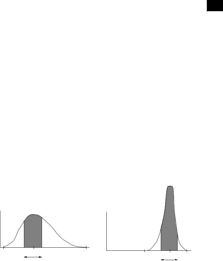
Metric Databases
d(q,u) ≤ r}, which retrieves all database elements at
distance at most r to q; and a k nearest neighbor query nnk
(q) = {ui U: vΥ, d(q,uι)≤ d(q,v) and |{υι }| = k}, which retrieves the k database elements closest to q.
Any such query can be answered by comparing the query q against the whole database, that is, computing d(q,u) for every u U. Because this is prohibitive, indexing techniques have been proposed to save as many distance computations as possible. Depending on the application, attention must also be paid to I/O costs and other CPU costs beyond computing distances.
There are some proximity searching problems in which a distance cannot be defined. Instead, a (dis)similarity is defined, which is a function not obeying the triangle inequality. It is common that the dissimilarity obeys a relaxed version of the triangle inequality, namely d(x,y) ≤ ν(d(x,z) + d(z,y)), with ν ≥ 1 and with probability ε > 0. Those cases can be dealt with by variants of the techniques used for metric spaces. If we cannot have even the relaxed version of the triangle inequality, then no better-than-brute-force approaches can be used.
THE CURSE OF DIMENSIONALITY
Vector spaces, typically using Euclidean distance, can be seen as metric spaces where objects are arrays of numbers. There exist many indexing mechanisms specifically aimed at indexing vector spaces (Gaede & Günther, 1998). In general, these mechanisms obtain better per-
formance than general metric space indexes, especially
when the space has few coordinates. However, the situ- M ation gets more complicated with higher dimensional
spaces (Böhm, Berchtold, & Keim, 2001).
It is well known that the performance of any indexing algorithm on a uniformly distributed vector space will suffer from an exponential dependency on the dimension of the space. A random query with nonempty outcome will force any index to scan the whole database, rendering it useless. This is called the “curse of dimensionality,” and it makes uniformly distributed spaces of dimensions 20 or more, intractable in practice. On the other hand, if the data points are not uniformly distributed in the space, then some indexes are able to perform better by mapping the space to fewer dimensions without significantly losing distance information. The reason is that the representational dimension of the space (i.e., the number of coordinates) can be much larger than the intrinsic dimension, which is, intuitively, the lowest dimension from which the data points could be properly represented.
One of the benefits of seeing a vector space as a metric space is that the performance of the indexes directly depends on the intrinsic rather than the representational dimension, without need of any mapping. Even in metric spaces, where there is no notion of coordinates, there are spaces that are intrinsically more difficult to search than others, independent of the indexing method used. In order to accurately predict the achievable performance of searching a given metric space and to apply the most adequate index given its intrinsic difficulty, it is important to be able to quantify
Figure 1. A low-dimensional (left) and high-dimensional (right) histogram of distances, showing that on high dimensions virtually all the elements become candidates for exhaustive evaluation
|
D PX |
|
D PX |
D PQ |
D PQ |
|
|
R |
R |
|
|
|
369 |
|
TEAM LinG |