

Kahan W.Lecture notes on IEEE standard 754 for binary floating-point arithmetic.1997
.pdfWork in Progress: |
Lecture Notes on the Status of IEEE 754 |
October 1, 1997 3:36 am |
|||
The first example shows how |
Infinity eases the numerical solution of a differential equation that appears to have |
||||
no divisions in it. The problem is to compute |
y(10) |
where y(t) satisfies the Riccati |
equation |
||
|
dy/dt = |
t + y2 |
for all t ³ 0 , |
y(0) = 0 . |
|
Let us pretend not to know that y(t) may be expressed in terms of |
Bessel functions |
J... , whence |
|||
y(10) = -7.53121 10731 35425 34544 97349 58··· . |
Instead a numerical method will be used to solve the |
||||
differential equation approximately and as accurately as desired if enough time is spent on it. |
|||||
Q(q, t, Y) will stand for an Updating Formula that advances from any estimate Y » y(t) to a later estimate Q(q, t, Y) » y(t+q) . Vastly many updating formulas exist; the simplest that might be applied to solve the given Riccati equation would be Euler's formula:
Q(q, t, Y) := Y + q·(t + Y2) .
This “ First-Order ” formula converges far too slowly as stepsize q |
shrinks; a faster “ Second-Order ” formula, |
|
of Runge-Kutta type, is Heun's : |
|
|
f := t + Y2 ; |
q := Y + q·f ; |
|
Q(q, t, Y) := Y + ( f + t+q + q2 )·q/2 .
Formulas like these are used widely to solve practically all ordinary differential equations. Every updating formula
is intended to be iterated with a sequence of stepsizes |
q that add up to the distance to be covered; for instance, |
|||||||||
Q(...) may be iterated |
N times with constant stepsize |
q := 10/N |
to produce |
Y(n·q) » y(n·q) thus: |
||||||
|
|
Y(0) := y(0) ; |
Y(n·q) := |
Q( q, (n-1)·q, Y((n-1)·q) ) . |
|
|||||
|
|
for |
n = 1 to N do |
|
||||||
Here the number N of |
timesteps |
is chosen with a view to the desired accuracy since the error |
Y(10) - y(10) |
|||||||
normally approaches 0 as N increases to Infinity. Were Euler's formula used, |
the error in its final estimate |
|||||||||
Y(10) would normally decline as fast as 1/N ; |
were Heun's, ... 1/N2 . But the Riccati |
differential equation is |
||||||||
not normal; no matter how big the number N |
of steps, those formulas’ estimates |
Y(10) |
turn out to be huge |
|||||||
positive numbers or overflows instead of -7.53··· . Conventional updating formulas do not work here. |
||||||||||
The simplest unconventional updating formula |
Q available turns out to be this rational formula: |
|
||||||||
Q(q, t, Y) |
:= |
Y + (t + --1 q + |
Y2)·q/( 1 - q·Y ) |
if |
|
1 |
, |
|||
|q·Y| < -- |
||||||||||
|
|
|
|
2 |
|
|
|
|
2 |
|
|
|
:= |
|
1 |
|
|
otherwise. |
|
||
|
|
( 1/q + (t + -- q)·q )/( 1 - q·Y ) - 1/q |
|
|||||||
|
|
|
|
2 |
|
|
|
|
|
|
The two algebraically equivalent forms are distinguished to curb rounding errors. Like Heun's, |
this Q is a second- |
|||||||||
order formula. ( It can be compounded into a formula of arbitrarily high order by means that lie beyond the scope of these notes.) Iterating it N times with stepsize q := 10/N yields a final estimate Y(10) in error by roughly
(105/N)2 even if Division-by-Zero insinuates an Infinity among the iterates Y(n·q) . Disallowing Infinity and Division-by-Zero would at least somewhat complicate the estimation of y(10) because y(t) has to pass through Infinity seven times as t increases from 0 to 10 . ( See the graph on the next page.)
What becomes complicated is not the program so much as the process of developing and verifying a program that
can dispense with Infinity. First, find a very tiny number e barely small enough that |
1 + 10 Öe rounds off to |
||
1 . Next, modify the foregoing rational formula for Q by replacing the divisor |
( 1 - q·Y ) in the “ otherwise ” |
||
case by ( ( 1 - q·Y ) + e ) |
. Do not omit any of these parentheses; they prevent divisions by zero. Then perform |
||
an error-analysis to confirm that iterating this formula produces the same values |
Y(n·q) |
as would be produced |
|
without e except for replacing infinite values Y by huge finite values. |
|
|
|
Survival without Infinity |
is always possible since “ Infinity ” is just a short word for a lengthy explanation. The |
||
price paid for survival without Infinity is lengthy cogitation to find a not-too-lengthy substitute, if it exists.
Page 11
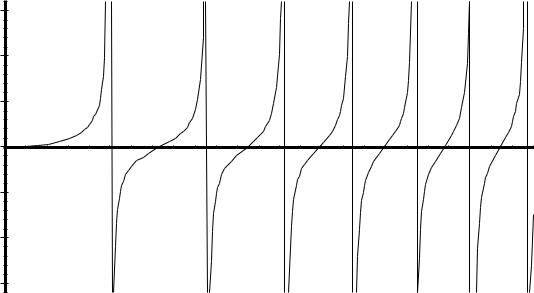
Work in Progress: |
Lecture Notes on the Status of IEEE 754 |
October 1, 1997 3:36 am |
.
Maple V r3 |
plots the solution |
y(t) |
of a |
Riccati |
equation |
|
15 |
|
|
|
|
|
|
10 |
|
|
|
|
|
|
5 |
|
|
|
|
|
|
0 |
2 |
4 |
6 |
|
8 |
10 |
|
|
t |
|
|
|
|
-5 |
|
|
|
|
|
|
-10 |
|
|
|
|
|
|
-15 |
|
|
|
|
|
|
End of first example.
The second example that illustrates the utility of Infinity is part of the fastest program known for computing a few eigenvalues of a real symmetric matrix. This part can be programmed to run well on every commercially significant computer that conforms to IEEE 754, but not in any single higher-level language that all such computers recognize.
|
|
|
|
|
|
|
|
|
|
|
a[1] b[2] |
|
|
|
|
No b [ j ] = 0 . |
|
||
|
b[2] a[2] b[3] |
|
|
|
|
|
|||
|
|
|
|
|
|
|
|
||
Let T = |
|
b[3] a[3] b[4] |
|
. |
Let q [1] := |
0 |
and |
||
|
b[4] a[4 |
] |
¼ |
|
|
|
|
|
|
|
|
|
|
q [ j ] := b [ j ]2 > 0 |
|||||
|
¼ |
|
¼ b[n ] |
|
|||||
|
|
|
|
|
≤ n . |
||||
|
|
|
|
b[n ] a[n ] |
|
for |
1 <j |
||
|
|
|
|
|
|
||||
Every real symmetric matrix reduces quickly to a tridiagonal form like |
T with the same eigenvalues |
||||||||
τ[1] < τ[2] < ... < τ[n] . The task is to find some of them specified either by an interval in which they lie or by their indices. Typically a few dozen eigenvalues may be sought when the dimension n is in the thousands. For this task the fastest and most accurate algorithm known is based upon the properties of two functions f = f (σ) and
k = k(σ) defined for real variable σ thus:
σ := σ + 0 ; |
|
| |
If σ = 0 , this ensures it is +0 , |
|
k := n ; |
f := 1 ; |
|
| |
|
FOR j |
= 1, 2, 3, ..., n IN TURN, |
|
| |
|
DO { |
f := ( σ - a [ j ] ) - q [ j ]/f |
; |
| |
Note: This loop has no explicit |
|
k := k - SignBit(f ) |
} ; |
| |
tests nor branches. |
k(σ) := k ; f (σ) := f . |
|
| |
|
|
Page 12
Work in Progress: |
|
Lecture Notes on the Status of IEEE 754 |
October 1, 1997 3:36 am |
||||||||
( The function |
SignBit(f ) := |
0 |
if f |
> 0 |
or |
if |
f |
is |
+0 or -0 , |
|
|
|
|
:= |
1 |
if |
f < 0 |
or |
if |
f is -0 ; |
|
||
its value at f |
= -0 may not matter but its value at |
f |
= -∞ |
does. It can be computed by using logical right-shifts |
|||||||
or by using |
|
|
|
|
|
|
|
|
|
|
|
|
( f |
< 0.0 ) |
|
|
in |
C , |
or |
|
|
|
|
|
0.5 |
- SIGN(0.5, f ) |
|
in |
Fortran, |
or |
|
||||
|
0.5 |
- CopySign(0.5, f ) |
from IEEE 754 . |
|
|||||||
However, the use of shifts or CopySign is mandatory on computers that depart from IEEE 754 |
by flushing |
|
UNDERFLOWed subtractions to -0.0 instead of UNDERFLOWing Gradually, q. v. below. |
|
|
Through an unfortunate accident, the arguments of |
CopySign are reversed on Apple computers, which otherwise |
|
conform conscientiously to IEEE 754; they require |
SignBit( f) := 0.5 - CopySign(f , 0.5) |
.) |
f (s) = s |
– a[n] – |
b[n]2 |
. |
b[n – 1]2 - |
|||
The function f (σ) is a |
-------------------------------------------------------------------------------------------------------s – a[n – 1] – |
- |
|
continued fraction: |
|
|
s – a[n – 2] – |
b[n – 2]2 |
|
-------------------------------------------------------------------b[2]2 |
||
|
||
|
s – a[n – 3] – ¼ – s-------------------– a[1] |
The eigenvalues τ[j] of T are the zeros of f (σ) , separated by the poles of f (σ) at which it interrupts its monotonic increasing behavior to jump from +∞ to -∞. The integer function k(σ) counts the eigenvalues on either side of σ thus:
τ[1] < τ[2] < ... < τ[k(σ)] |
≤ |
σ < |
τ[k(σ)+1] |
< ... < τ[n] , and |
τ[k(σ)] |
= |
σ |
just when |
f (σ) = 0 . |
Evidently the eigenvalues τ[j] of T are the n values of σ at which k(σ) jumps, and may be located by Binary Search accelerated by interpolative schemes that take values of f (σ) into account too. Although rounding errors can obscure f (σ) severely, its monotonicity and the jumps of k(σ) are practically unaffected, so the eigenvalues are obtained more accurately this way than any other. And quickly too.
If Infinity were outlawed, the loop would have to be encumbered by a test and branch to prevent Division-by- Zero. That test cannot overlap the division, a slow operation, because of sequential dependencies, so the test would definitely slow down the loop even though zero would be detected extremely rarely. The test's impact would be tolerable if the loop contained only one division, but that is not what happens.
Because division is so slow, fast computers pipeline it in such a way that a few divisions can be processed concurrently. To exploit this pipelining, we search for several eigenvalues simultaneously. The variable σ becomes a small array of values, as do f and k , and every go-around the loop issues an array of divisions. In this context the tests, though “ vectorized ” too, degrade speed by 25% or more, much more on machines with multiple pipelines that can subtract and shift concurrently with division, regardless of what else a branch would entail whenever a zero divisor were detected. By dispensing with those tests, this program gains speed and simplicity from Infinity even if Division-by-Zero never happens.
End of second example.
How many such examples are there? Nobody knows how many programs would benefit from Infinity because it remains unsupported by programming language standards, and hence by most compilers, though support in hardware has been abundant for over a decade. To get some idea of the impediment posed by lack of adequate support, try to program each of the foregoing two examples in a way that will compile correctly on every machine whose hardware conforms to IEEE 754. That ordeal will explain why few programmers experiment with Infinity, whence few programs use it.
Page 13
Work in Progress: Lecture Notes on the Status of IEEE 754 October 1, 1997 3:36 am
In my experience with a few compilers that support IEEE 754 on PCs and Macintoshes, Infinity and NaNs confer their greatest benefits by simplifying test programs, which already tend to grossly worse complexity than the software they are designed to validate. Consequently my programs enjoy enhanced reliability because of IEEE 754 regardless of whether it is in force where they run.
...... End of Digression ......
Exception: OVERFLOW.
This happens after an attempt to compute a finite result that would lie beyond the finite range of the floating-point format for which it is destined. The default specified in IEEE 754 is to approximate that result by an appropriately signed Infinity. Since it is approximate, OVERFLOW is also INEXACT. Often that approximation is worthless; it is almost always worthless in matrix computations, and soon turns into NaN or, worse, misleading numbers. Consequently OVERFLOW is often trapped to abort seemingly futile computation sooner rather than later.
Actually, OVERFLOW more often implies that a different computational path should be chosen than that no path leads to the desired goal. For example, if the Fortran expression x / SQRT(x*x + y*y) encounters OVERFLOW before the SQRT can be computed, it should be replaced by something like
(s*x) / SQRT( (s*x)*(s*x) + (s*y)*(s*y) )
with a suitably chosen tiny positive Scale-Factor s . ( A power of 2 avoids roundoff.) The cost of computing and applying s beforehand could be deemed the price paid for insurance against OVERFLOW. Is that price too high?
The biggest finite IEEE 754 Double is almost 1.8 e308 , which is so huge that OVERFLOW occurs extremely rarely if not yet rarely enough to ignore. The cost of defensive tests, branches and scaling to avert OVERFLOW seems too high a price to pay for insurance against an event that hardly ever happens. A lessened average cost will be incurred in most situations by first running without defensive scaling but with a judiciously placed test for OVERFLOW ( and for severe UNDERFLOW ); in the example above the test should just precede the SQRT. Only when necessary need scaling be instituted. Thus our treatment of OVERFLOW has come down to this question: how best can OVERFLOW be detected?
The ideal test for OVERFLOW tests its flag; but that flag cannot be mentioned in most programming languages for lack of a name. Next best are tests for Infinities and NaNs consequent upon OVERFLOW, but prevailing
programming languages lack names for them; suitable tests have to be contrived. For example, the |
C predicate |
||
(z != z) is True |
only when z is NaN |
and the compiler has not “ optimized ” overzealously; |
|
(1.0e37 /(1 + fabs(z)) == 0) is |
True only when z is infinite; and (z-z != 0) is |
True only |
|
when z is NaN or |
infinite, the INVALID |
trap has been disabled, and optimization is not overzealous. |
|
A third way to detect |
OVERFLOW is to enable its trap and attach a handler to it. Even if a programming |
||
language in use provides control structures for this purpose, this approach is beset by hazards. The worst is the possibility that the handler may be entered inadvertently from unanticipated places. Another hazard arises from the concurrent execution of integer and floating-point operations; by the time an OVERFLOW has been detected, data associated with it may have become inaccessible because of changes in pointers and indices. Therefore this approach works only when a copy of the data has been saved to be reprocessed by a different method than the one thwarted by OVERFLOW, and when the scope of the handler has been properly localized; note that the handler must be detached before and reattached after functions that handle their own OVERFLOWs are executed.
The two costs, of saving and scoping, must be paid all the time even though OVERFLOW rarely occurs. For these reasons and more, other approaches to the OVERFLOW problem are to be preferred, but a more extensive discussion of them lies beyond the intended scope of this document.
Page 14
Work in Progress: |
Lecture Notes on the Status of IEEE 754 |
October 1, 1997 3:36 am |
When OVERFLOW's trap is enabled, the IEEE 754 default Infinity is not generated; instead, the result's exponent is “ wrapped,” which means in this case that the delivered result has an exponent too small by an
amount 2K-1·3 that depends upon its format:
Double-Extended |
... too small by |
24576 ; 224576 = 1.3 E 7398 |
||
Double |
... too small by |
1536 |
; |
21536 = 2.4 E 462 |
Single |
... too small by |
192 |
; |
2192 = 6.3 E 57 |
( Though required by |
IEEE 754, the latter two are not performed by |
ix87 nor 680x0 |
||
nor some other machines without help from suitable trap-handling software. )
In effect, the delivered result has been divided by a power of 2 so huge as to turn what would have overflowed into a relatively small but predictable quantity that a trap-handler can reinterpret. If there is no trap handler, computation will proceed with that smaller quantity or, in the case of format-converting FSTore instructions, without storing anything. The reason for exponent wrapping is explained after UNDERFLOW.
Exception: UNDERFLOW.
This happens after an attempt to approximate a nonzero result that lies closer to zero than the intended floatingpoint destination's “ Normal ” positive number nearest zero. 2.2 e-308 is that number for IEEE 754 Double. A nonzero Double result tinier than that must by default be rounded to a nearest Subnormal number, whose magnitude can run from 2.2 e-308 down to 4.9 e-324 ( but with diminishing precision ), or else by 0.0 when no Subnormal is nearer. IEEE 754 Extended and Single formats have different UNDERFLOW thresholds, for which see the table “ Span and Precision of IEEE 754 Floating-Point Formats ” above. If that rounding incurs no error, no UNDERFLOW is signaled.
Subnormal numbers, also called “ Denormalized,” allow UNDERFLOW to occur Gradually; this means that gaps between adjacent floating-point numbers do not widen suddenly as zero is passed. That is why Gradual UNDERFLOW incurs errors no worse in absolute magnitude than rounding errors among Normal numbers. No such property is enjoyed by older schemes that, lacking Subnormals, flush UNDERFLOW to zero abruptly and suffer consequent anomalies more fundamental than afflict Gradual UNDERFLOW.
For example, the C predicates x == y and x-y == 0 are identical in the absence of OVERFLOW only if UNDERFLOW is Gradual. That is so because x-y cannot UNDERFLOW Gradually; if x-y is Subnormal then it is Exact. Without Subnormal numbers, x/y might be 0.95 and yet x-y could UNDERFLOW abruptly to 0.0 , as could happen for x and y tinier than 20 times the tiniest nonzero Normal number. Consequently, Gradual Underflow simplifies a theorem very important for the attenuation of roundoff in numerical computation:
If p |
and |
q are floating-point numbers in the same format, and if |
1/2 ≤ p/q ≤ 2 |
, |
then |
p - q |
is computable exactly ( without a rounding error ) in that format. But |
||
if UNDERFLOW is not Gradual, and if p - q UNDERFLOWs, |
it is not exact. |
|
||
More generally, floating-point error-analysis is simplified by the knowledge, first, that IEEE 754 rounds every finite floating-point result to its best approximation by floating-point numbers of the chosen destination's format, and secondly that the approximation's absolute uncertainty ( error bound ) cannot increase as the result diminishes in magnitude. Error-analysis, and therefore program validation, is more complicated, sometimes appallingly more so, on those currently existing machines that do not UNDERFLOW Gradually.
Though afflicted by fewer anomalies, Gradual UNDERFLOW is not free from them. For instance, it is possible to have x/y == 0.95 coexist with (x*z)/(y*z) == 0.5 because x*z and probably also y*z UNDERFLOWed to Subnormal numbers; without Subnormals the last quotient turns into either an ephemeral 0.0 or a persistent NaN ( INVALID 0/0 ). Thus, UNDERFLOW cannot be ignored entirely whether Gradual
Page 15
Work in Progress: |
Lecture Notes on the Status of IEEE 754 |
October 1, 1997 3:36 am |
or not.
UNDERFLOWs are uncommon. Even if flushed to zero they rarely matter; if handled Gradually they cause harm extremely rarely. That harmful remnant has to be treated much as OVERFLOWs are, with testing and scaling, or trapping, etc. However, the most common treatment is to ignore UNDERFLOW and then to blame whatever harm is caused by doing so upon poor taste in someone else's choice of initial data.
UNDERFLOWs resemble ants; where there is one there are quite likely many more, and they tend to come one after another. That tendency has no direct effect upon the i387-486-Pentium nor M68881/2, but it can severely retard computation on other implementations of IEEE 754 that have to trap to software to UNDERFLOW Gradually for lack of hardware to do it. They take extra time to Denormalize after UNDERFLOW and/or, worse, to prenormalize Subnormals before multiplication or division. ( Gradual UNDERFLOW requires no prenormalization before addition or subtraction of numbers with the same format, but computers usually do it anyway if they have to trap Subnormals.) Worse still is the threat of traps, whether they occur or not, to machines like the DEC Alpha that cannot enable traps without hampering pipelining and/or concurrency; such machines are slowed also by Gradual UNDERFLOWs that do not occur!
Why should we care about such benighted machines? They pose dilemmas for developers of applications software designed to be portable (after recompilation) to those machines as well as ours. To avoid sometimes severe performance degradation by Gradual UNDERFLOW, developers will sometimes resort to simple-minded alternatives. The simplest violates IEEE 754 by flushing every UNDERFLOW to 0.0 , and computers are being sold that flush by default. ( DEC Alpha is a recent example; it is advertised as conforming to IEEE 754 without mention of how slowly it runs with traps enabled for full conformity.) Applications designed with flushing in mind may, when run on ix87s and Macs, have to enable the UNDERFLOW trap and provide a handler that flushes to zero, thereby running slower to get generally worse results! ( This is what MathCAD does on PCs and on Macintoshes.) Few applications are designed with flushing in mind nowadays; since some of these might malfunction if UNDERFLOW were made Gradual instead, disabling the ix87 UNDERFLOW trap to speed them up is not always a good idea.
A format’s usable exponent range is widened by almost its precision N to fully ±2 K as a by-product of Gradual Underflow; were this its sole benefit, its value to formats wider than Single could not justify its price. Compared with Flush-to-Zero, Gradual Underflow taxes performance unless designers expend time and ingenuity or else hardware. Designers incapable of one of those expenditures but willing to cut a corner off IEEE 754 exacerbate market fragmentation, which costs the rest of us cumulatively far more than whatever they saved.
...... Digression on Gradual Underflow ......
To put things in perspective, here is an example of a kind that, when it appears in benchmarks, scares many people into choosing Flush-to-Zero rather than Gradual UNDERFLOW. To simulate the diffusion of heat through a conducting plate with edges held at fixed temperatures, a rectangular mesh is drawn on the plate and temperatures are computed only at intersections. The finer the mesh, the more accurate is the simulation. Time is discretized too; at each timestep, temperature at every interior point is replaced by a positively weighted average of that point's temperature and those of nearest neighbors. Simulation is more accurate for smaller timesteps, which entail larger numbers of timesteps and tinier weights on neighbors; typically these weights are smaller than 1/8 , and timesteps number in the thousands.
When edge temperatures are mostly fixed at 0 , and when interior temperatures are mostly initialized to 0 , then at every timestep those nonzero temperatures next to zeros get multiplied by tiny weights as they diffuse to their neighbors. With fine meshes, large numbers of timesteps can pass before nonzero temperatures have diffused almost everywhere, and then tiny weights can get raised to large powers, so UNDERFLOWs are numerous. If
Page 16
Work in Progress: |
Lecture Notes on the Status of IEEE 754 |
October 1, 1997 3:36 am |
UNDERFLOW is Gradual, denormalization will produce numerous subnormal numbers; they slow computation badly on a computer designed to handle subnormals slowly because the designer thought they would be rare. Flushing UNDERFLOW to zero does not slow computation on such a machine; zeros created that way may speed it up.
When this simulation figures in benchmarks that test computers' speeds, the temptation to turn slow Gradual UNDERFLOW Off and fast Flush-to-Zero On is more than a marketing manager can resist. Compiler vendors succumb to the same temptation; they make Flush-to-Zero their default. Such practices bring to mind calamitous explosions that afflicted high-pressure steam boilers a century or so ago because attendants tied down noisy overpressure relief valves the better to sleep undisturbed.
+ |
--------------------------------------------------------------------- |
|
|
|
|
|
|
|
+ |
| |
Vast numbers |
of |
UNDERFLOWs usually |
signify that something |
about |
| |
|||
| |
a program or |
its |
data |
is strange if not |
wrong; |
this signal |
should | |
||
| |
not be ignored, |
much |
less squelched |
by |
flushing |
UNDERFLOW |
to |
0.| |
|
+--------------------------------------------------------------------- |
|
|
|
|
|
|
|
|
+ |
What is strange about the foregoing simulation is that exactly zero temperatures occur rarely in Nature, mainly at the boundary between colder ice and warmer water. Initially increasing all temperatures by some negligible
amount, say 10-30 , would not alter their physical significance but it would eliminate practically all UNDERFLOWs and so render their treatment, Gradual or Flush-to-Zero, irrelevant.
To use such atypical zero data in a benchmark is justified only if it is intended to expose how long some hardware takes to handle UNDERFLOW and subnormal numbers. Unlike many other floating-point engines, the i387 and its successors are slowed very little by subnormal numbers; we should thank Intel's engineers for that and enjoy it rather than resort to an inferior scheme which also runs slower on the i387-etc.
...... End of Digression ......
When UNDERFLOW's trap is enabled, the IEEE 754 default Gradual Underflow does not occur; the result's exponent is “ wrapped ” instead, which means in this case that the delivered result has an exponent too big by an
amount 2K-1·3 that depends upon its format:
Double-Extended |
... too big by |
24576 ; |
224576 = 1.3 E 7398 |
|
Double |
... too big by |
1536 |
; |
21536 = 2.4 E 462 |
Single |
... too big by |
192 |
; |
2192 = 6.3 E 57 |
( Though required by |
IEEE 754, the latter two wraps are not performed by ix87 nor 680x0 |
|||
nor some other machines without help from suitable trap-handling software. )
In effect, the delivered result has been multiplied by a power of 2 so huge as to turn what would have underflowed into a relatively big but predictable quantity that a trap-handler can reinterpret. If there is no trap handler, computation will proceed with that bigger quantity or, in the case of format-converting FSTore instructions, without storing anything.
Exponent wrapping provides the fastest and most accurate way to compute extended products and quotients like
(a1 + b1 ) × (a2 + b2 ) × (a3 + b3 ) × (¼) × (aN + bN )
Q = ----------------------------------------------------------------------------------------------------------------------
(c1 + d1 ) × (c2 + d2 ) × (c3 + d3 ) × (¼) × (cM + dM )
when N and M are huge and when the numerator and/or denominator are likely to encounter premature OVER/ UNDERFLOW even though the final value of Q would be unexceptional if it could be computed. This situation arises in certain otherwise attractive algorithms for calculating eigensystems, or Hypergeometric series, for example.
Page 17
Work in Progress: |
Lecture Notes on the Status of IEEE 754 |
October 1, 1997 3:36 am |
What Q requires is an OVER/UNDERFLOW trap-handler that counts OVERFLOWs and UNDERFLOWs but leaves wrapped exponents unchanged during each otherwise unaltered loop that computes separately the numerator's and denominator's product of sums. The final quotient of products will have the correct significant bits but an exponent which, if wrong, can be corrected by taking counts into account. This is by far the most satisfactory way to compute Q , but for lack of suitable trap-handlers it is hardly ever exploited though it was implemented on machines as diverse as the IBM 7094 and /360 ( by me in Toronto in the 1960s; see Sterbenz
(1974) ), a Burroughs B5500 ( by Michael Green |
at Stanford in 1966 ), and a DEC VAX ( in 1981 by |
David Barnett, then an undergraduate at Berkeley ). |
Every compiler seems to require its own implementation. |
Exception: INEXACT.
This is signaled whenever the ideal result of an arithmetic operation would not fit into its intended destination, so the result had to be altered by rounding it off to fit. The INEXACT trap is disabled and its flag ignored by almost all floating-point software. Its flag can be used to improve the accuracy of extremely delicate approximate computations by “ Exact Preconditioning,” a scheme too arcane to be explained here; for an example see pp. 107110 of Hewlett-Packard’s HP-15C Advanced Functions Handbook (1982) #00015-90011. Another subtle use for the INEXACT flag is to indicate whether an equation f(x) = 0 is satisfied exactly without roundoff ( in which case x is exactly right ) or despite roundoff ( in which not–so–rare case x may be arbitrarily erroneous ).
A few programs use REAL variables for integer arithmetic. M680x0s and ix87s can handle integers up to 65 bits wide including sign, and convert all narrower integers to this format on the fly. In consequence, arithmetic with wide integers may go faster in floating-point than in integer registers at most 32 bits wide. But then when an integer result gets too wide to fit exactly in floating-point it will be rounded off. If this rounding went unnoticed it could lead to final results that were all unaccountably multiples of, say, 16 for lack of their last few bits. Instead, the INEXACT exception serves in lieu of an INTEGER OVERFLOW signal; it can be trapped or flagged.
Well implemented Binary-Decimal conversion software signals INEXACT just when it is deserved, just as rational operations and square root do. However, an undeserved INEXACT signal from certain transcendental functions like X**Y when an exact result is delivered accidentally can be very difficult to prevent.
Directions of Rounding:
The default, reset by turning power off-on, rounds every arithmetic operation to the nearest value allowed by the assigned precision of rounding. When that nearest value is ambiguous ( because the exact result would be one bit wider than the precision calls for ) the rounded result is the “ even ” one with its last bit zero. Note that rounding to the nearest 16-, 32or 64-bit integer ( float-to-int store ) in this way takes both 1.5 and 2.5 to 2 , so the various INT, IFIX, ... conversions to integer supported by diverse languages may require something else. One of my Fortran compilers makes the following distinctions among roundings to nearest integers:
IRINT, RINT, DRINT |
round to nearest even, as ix87 FIST does. |
NINT, ANINT, DNINT round half-integers away from 0 . |
|
INT, AINT, DINT |
truncate to integers towards 0 . |
Rounding towards 0 causes subsequent arithmetic operations to be truncated, rather than rounded, to the nearest value in the direction of 0.0 . In this mode, store-to-int provides INT etc. This mode also resembles the way many old machines now long gone used to round.
Page 18
Work in Progress: |
Lecture Notes on the Status of IEEE 754 |
October 1, 1997 3:36 am |
The “ Directed ” roundings can be used to implement Interval Arithmetic, which is a scheme that approximate every variable not by one value of unknown reliability but by two that are guaranteed to straddle the ideal value. This scheme is not so popular in the U.S.A. as it is in parts of Europe, where some people distrust computers.
Control-Word control of rounding modes allows software modules to be re-run in different rounding modes without recompilation. This cannot be done with some other computers, notably DEC Alpha, that can set two bits in every instruction to control rounding direction at compile-time; that is a mistake. It is worsened by the designers' decision to take rounding direction from a Control-Word when the two bits are set to what would otherwise have been one of the directed roundings; had Alpha obtained only the round-to-nearest mode from the Control-Word, their mistake could have been transformed into an advantageous feature.
All these rounding modes round to a value drawn from the set of values representable either with the precision of the destination or selected by rounding precision control to be described below. The sets of representable values were spelled out in tables above. The direction of rounding can also affect OVER/UNDERFLOW ; a positive quantity that would OVERFLOW to +∞ in the default mode will turn into the format's biggest finite floatingpoint number when rounded towards -∞. And the expression “ X - X ” delivers +0.0 for every finite X in all rounding modes except for rounding directed towards -∞, for which -0.0 is delivered instead. These details are designed to make Interval Arithmetic work better.
Ideally, software that performs Binary-Decimal conversion ( both ways ) should respect the requested direction
of rounding. David Gay of AT&T Bell Labs |
has released algorithms that do so into the public domain ( Netlib ); |
to use less accurate methods now is a blunder. |
|
Precisions of Rounding:
IEEE 754 obliges only machines that compute in the Extended ( long double or REAL*10 ) format to let programmers control the precision of rounding from a Control-Word. This lets ix87 or M680x0 emulate the roundoff characteristics of other machines that conform to IEEE 754 but support only Single ( C's float, or REAL*4 ) and Double ( C's double, or REAL*8 ), not Extended. Software developed and checked out on one of those machines can be recompiled for a 680x0 or ix87 and, if anomalies excite concerns about differences in roundoff, the software can be run very nearly as if on its original host without sacrificing speed on the 680x0
or ix87. Conversely, software developed on these machines but without explicit mention of Extended can be rerun in a way that portends what it will do on machines that lack Extended. Precision Control rounds to 24 sig. bits to emulate Single, to 53 sig. bits to emulate Double, leaving zeros in the rest of the 64 sig. bits of the Extended format.
The emulation is imperfect. Transcendental functions are unlikely to match. Although Decimal -> Binary conversion must round to whatever precision is set by the Control-Word, Binary -> Decimal should ideally be unaffected since its precision is determined solely by the destination’s format, but ideals are not always attained. Some OVER/UNDERFLOWs that would occur on those other machines need not occur on the ix87 ; IEEE 754 allows this, perhaps unwisely, to relieve hardware implementors of details formerly thought unimportant.
Few compilers expose the Control-Word to programmers. Worse, some compilers have revived a nasty bug that emerged when Double-Precision first appeared among Fortran compilers; it goes like this: Consider
S = X
T = ( S - Y )/( . . . )
in a Fortran program where S is SINGLE PRECISION, and X and Y are DOUBLE or EXTENDED PRECISION variables or expressions computed in registers. Compilers that supplant S by X in the second statement save the time required to reload S from memory but spoil T . Though S and X differ by merely a rounding error, the difference matters.
Page 19
Work in Progress: |
Lecture Notes on the Status of IEEE 754 |
October 1, 1997 3:36 am |
The Baleful Influence of Benchmarks:
Hardware and compilers are increasingly being rated entirely according to their performance in benchmarks that measure only speed. That is a mistake committed because speed is so much easier to measure than other qualities like reliability and convenience. Sacrificing them in order to run faster will compel us to run longer. By disregarding worthwhile qualities other than speed, current benchmarks penalize conscientious adherence to standards like IEEE 754; worse, attempts to take those qualities into account are thwarted by political constraints imposed upon programs that might otherwise qualify as benchmarks.
For example, a benchmark should compile and run on every commercially significant computer system. This rules out our programs for solving the differential equation and the eigenvalue problem described above under the Digression on Division-by-Zero. To qualify as benchmarks, programs must prevent exceptional events that might stop or badly slow some computers even if such prevention retards performance on computers that, by conforming conscientiously to IEEE 754, would not stop.
The Digression on Gradual Underflow offered an example of a benchmark that lent credibility to a misguided preference for Flush-to-Zero, in so far as it runs faster than Gradual Underflow on some computers, by disregarding accuracy. If Gradual Underflow's superior accuracy has no physical significance there, neither has the benchmark's data.
Accuracy poses tricky questions for benchmarks. One hazard is the ...
Stopped Clock Paradox: Why is a mechanical clock more accurate stopped than running?
A running clock is almost never exactly right, whereas a stopped clock is exactly right twice a day. ( But WHEN is it right? Alas, that was not the question.)
The computational version of this paradox is a benchmark that penalizes superior computers, that produce merely excellent approximate answers, by making them seem less accurate than an inferior computer that gets exactly the right answer for the benchmark's problem accidentally. Other hazards exist too; some will be illustrated by the next example.
Quadratic equations like
p x2 - 2 q x + r = 0
arise often enough to justify tendering a program that solves it to serve as a benchmark. When the equation's roots x1 and x2 are known in advance both to be real, the simplest such program is the procedure Qdrtc exhibited on the next page.
In the absence of premature |
Over/Underflow, Qdrtc |
computes |
x1 and x2 at least about as accurately as they |
||
are determined by data { p, q, r } |
uncorrelatedly uncertain in their last digits stored. It should be tested first on |
||||
trivial data to confirm that it has not been corrupted by a misprint nor by an ostensible correction like |
|||||
“ x1 := (q+s)/p ; x2 := (q-s)/p ” |
copied naively from some elementary programming text. Here are some trivial |
||||
data: |
|
|
|
|
|
{ p = Any nonzero, q = r = 0 }; |
x1 = x2 = 0 . |
||||
{ p = 2.0 |
, |
q = 5.0 , r = 12.0 }; |
x1 = 2.0 , |
x2 = 3.0 . |
|
{ p = 2.0 |
E-37, |
q = 1.0 , r = 2.0 }; |
x1 ≈ 1.0 , x2 ≈ 1.0 E 37 . |
||
Swapping p with r swaps { x1, x2 } with { 1/x2, 1/x1 } .
{µ*p, µ*q, µ*r} yields {x1, x2} independently of nonzero µ .
Page 20