

Joye M.Cryptographic hardware and embedded systems.2005
.pdf156 |
R.M. Avanzi |
|
|
|
class represented by |
|
with Lange’s new co- |
||
ordinates |
[24], the sextuple |
corresponds to the ideal class |
||
|
|
|
The system |
is important in scalar |
multiplications since it has the fastest doubling. We refer to [24] for the formulae.
We now see in an example – the addition formula in affine coordinates – how lazy and incomplete reductions are used in practice. Table 3 is derived from results in [24], but restricted to the odd characteristic case. The detailed breakdown of the REDCs we can save follows:
1.In Step 1 we can save one REDC in the computation of  since we do not need the reduced value of
  and
and  anywhere else.
2.In Step 3 we do not reduce  since it is used in the computation of
  and
and  which are sums of products of two elements. So only 3 REDCs are required to implement Step 3: for
  and for the final results of
  and
and  This is a saving of two REDCs.
3.In Step 5, it would be desirable to leave the coefficients and
and  of
of unreduced, since they are used in the following two steps only in additions with other products of two elements. But
  is a problem: we cannot add reduced and unreduced
TEAM LinG
Aspects of Hyperelliptic Curves over Large Prime Fields |
157 |
quantities (see Remark 1). We circumvent this by computing the unreduced products  (in place of
  and
and  Two REDCs are saved.
4.In Step 6, it is  We need only one REDC to compute the (reduced) sum of the first four products: Note
that, at this point,  is already known and we already counted the saving of one REDC associated to it. So, we save a total of two REDCs.
Summarizing, for one addition in affine coordinates in the most common case, we need 12 Muls, 13 MulNoREDCs and 6 REDCs. Thus, we save 7REDCs.
We implemented addition and doubling in all coordinate systems. To speed up scalar multiplication, we also implemented addition in the cases where one of the two group elements to be added is given in  and the second summand and the result are both given either in
  or
or 
In Table 2 we write the operation counts of the implemented operations. The table contains also the counts for EC and genus 3 curves (see the next paragraph). The number of modular reductions is always significantly smaller than the number of multiplications.
Genus 3. Affine coordinates are the only coordinate system currently available for genus 3 curves. The formulae in [32,33] contain some errors in odd characteristic. We took the formulae of [40] – which are for general curves of the form  and have been implemented only in even characteristic with
  – and simplified them for the case of odd characteristic,
  and vanishing second most significant coefficient of
  A pleasant aspect of these formulae is that a large proportion of modular reductions can be saved: at least 21 in the addition and 14 in the doubling (see Table 2).
2.4 Scalar Multiplication
There are many methods for computing a scalar multiplication in a generic group, which
can be used for EC and HEC. See [15] for a survey. |
|
|
||
A simple method for computing |
for an integer and a ideal class D is based |
|||
on the binary representation of If |
|
where each |
or 1, then |
|
can be computed as |
|
|
|
|
This requires |
doublings and on average |
additions on the curve (the first |
||
addition is replaced by an assignment).
On EC and HEC, adding and subtracting an element have the same cost. Hence one
can use the non adjacent form (NAF) [34], which is an expansion |
with |
||
|
and |
This leads to a method needing |
doublings and on |
average |
additions or subtractions. |
|
|
A generalization of the NAF uses “sliding windows”: The wNAF [37,8] of the integer
is a representation |
|
where the integers |
satisfy the following two |
|
conditions: (i) either |
or |
is odd and |
(ii) of any |
consecutive |
coefficients |
at most one is nonzero. The 1NAF coincides with the NAF. |
|||
TEAM LinG
158 R.M. Avanzi
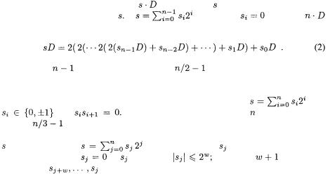
The wNAF has average density  To compute a scalar multiplication based on the wNAF one first precomputes the ideal classes D,
  and then performs a double-and-add step like (2). A left-to-right recoding with the same density as the wNAF can be found in [4].
3 Results, Comparisons, and Conclusions
Table 4 reports the timings of our implementation. Since nuMONGO provides support only for moduli up to 256 bits, EC are tested only on fields up to that size. For genus 2 curves on a 256 bit field, a group up to 513 bits is possible: We choose this group size as a limit also for the genus 3 curves.
All benchmarks were performed on a 1 GHz AMD Athlon (Model 4) PC, under the Linux operating system (kernel version 2.4). The compilers used were the GNU C Compiler (gcc), versions 2.95.3 and 3.3.1 and all the performance considerations made in § 2.1 apply.
All groups have prime or almost prime order. The elliptic curves up to 256 bits have been found by point counting on random curves, the larger ones as well as the genus 2 and 3 curves have been constructed with the CM method.
For each combination of curve type, coordinate system and group size, we averaged the timings of several thousands scalar multiplications with random scalars, using three different recodings of the scalar: the binary representation, the NAF, and the wNAF. For the wNAF we report only the best timing and the corresponding value of  We always keep the base ideal class and its multiples in affine coordinates, since adding an affine point to a point in any coordinate system other than affine is faster than adding two points in that coordinate system. The timings always include the precomputations.
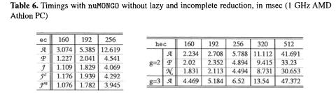
In Table 5 we provide timings for ecc and hec using gmp and the double-and-add scalar multiplication based on the unsigned binary representation. We also provide in Table 6 timings with nuMONGO but without lazy and incomplete reduction. For comparison with our timings, Lange [23] reported timings of 8.232 and 9.121 milliseconds for genus 2 curves with group  and
and  respectively on a gmp-based implementation of affine coordinates on a 1.5 GHz Pentium 4 PC. In [23] the double-and-add algorithm based on the unsigned binary representation is used. In [35], a timing of 98 milliseconds for a genus 3 curve of about 180 bits
  on an Alpha 21164A CPU running at 600MHz is reported. The speed of these two CPUs is close to that of the machine we used for our tests.
A summary of the results follows:
1.Using a specialized software library one can get a speed-up by a factor of 3 to 4.5 for EC with respect to a traditional implementation. The speed-up for genus 2 and 3 curves is up to 8.
2.Lazy and incomplete reduction bring a speed-up from 3% to 10%.
3.For EC, the performance of the systems  and
and  is almost identical. The reason lies in the fact that with
  no modular reductions can be saved.
4.HEC are still slower than EC, but the gap has been narrowed.
a)Affine coordinates for genus 2 HEC are significantly faster than those for EC. Those for genus 3 are faster from 144 bits upwards.
TEAM LinG

Aspects of Hyperelliptic Curves over Large Prime Fields |
159 |
TEAM LinG

 and
and are slower than
 because they require more function calls for each group operation than
 Therefore, with standard libraries the overheads can dominate the running time.
 there is a relative drop in performance with respect to other groups where the field size is almost a multiple of
  For example, a 160-bit group can be given by a genus 2 curve over a 80-bit field, but then 96-bit arithmetic must be used on a 32-bit CPU. Similarly, with 224-bit groups, a genus 2 HEC is penalized by the 112-bit field arithmetic. For 144-bit groups, genus 3 curves can exploit 48-bit arithmetic, which has been made faster by suitable implementation tricks (an approach which did not work for 80 and 112 bit fields), hence the gap to genus 2 is only 50%.
 Generic Efficient Arithmetic Algorithms for PAFFs (Processor Adequate Finite Fields) and Related Algebraic Structures.
 Special issue on Embedded Systems and Security of the ACM Transactions in Embedded Computing Systems.
 in round one will affect almost the entire second round. Detecting collisions by examining a sequence of instructions may be advantageous in terms of measurement costs. On the other hand, it must be noted that DPA based attacks against AES have the advantage of being known plaintext attacks whereas our proposed collision attack is a chosen plaintext attack.
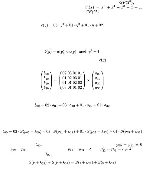
 The input polynomial is multiplied with the fixed polynomial
 elements 1,
  and
and  respectively. If we refer to the input column as
  and to the output column as
  the mix column transformation can be stated as
 it is given by
 and
and  with
with 
 and
and  The output byte
  can then be written as
 (or any other output byte of the mix column transformation) with side channel analysis. First, he sets the two plaintext bytes
  and
and  to a random value
  As next, he encrypts the corresponding plaintext, measures the power trace and stores it on his