
funct_m_q
.pdf
As a practical matter though, you'll probably be evaluating interp for many different points. The call to lspline can be time-consuming, and the result won't change from one point to the next, so do it just once and store the outcome in the vs array.
In addition to lspline, Mathcad comes with two other cubic spline functions for the twodimensional case: pspline and cspline. The pspline function generates a spline curve that approaches a second degree polynomial in x and y along the edges. The cspline function generates a spline curve that approaches a third degree polynomial in x and y along the edges.
Algorithm Tridiagonal system solving (Press et al., 1992; Lorczak)
lu
Syntax
Description
Arguments
(Professional) |
Vector and Matrix |
lu(M) |
|
Returns an n ´ (3 × n) |
matrix whose first n columns contain an n ´ n permutation matrix P, |
whose next n columns contain an n ´ n lower triangular matrix L, and whose remaining n columns contain an n ´ n upper triangular matrix U. These matrices satisfy the equation
P × M = L × U .
M real or complex n ´ n matrix
Comments This is known as the LU decompostion (or factorization) of the matrix M, permuted by P.
Algorithm Crout’s method with partial picoting (Press et al., 1992; Golub and Van Loan, 1989)
matrix
Syntax
Description
Arguments
Vector and Matrix
matrix(m, n, f)
Creates a matrix in which the ijth element is the value f(i, j), where i = 0, 1, ¼, m – 1 and j = 0, 1, ¼, n – 1 .
m, n |
integers |
f |
scalar-valued function |
|
|
max |
Vector and Matrix |
Syntax |
max(A) |
Description |
Returns the largest element in A. If A is complex, returns max(Re(A)) + i×max(Im(A)). |
Arguments |
|
A |
real or complex m ´ n matrix or vector |
See also |
min |
Functions |
61 |
Maximize
Syntax
Description
Arguments
Solving
Maximize(f, var1, var2,...)
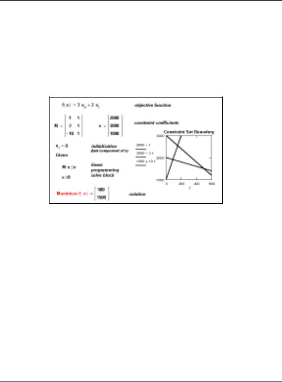
Returns values of var1, var2,... which solve a prescribed system of equations, subject to prescribed inequalities, and which make the function f take on its largest value. The number of arguments matches the number of unknowns, plus one. Output is a scalar if only one unknown; otherwise it is a vector of answers.
f real-valued objective function
var1, var2, ... real or complex variables; var1, var2,.. must be assigned guess values before using Maximize
Examples
62 |
Chapter 1 Functions |
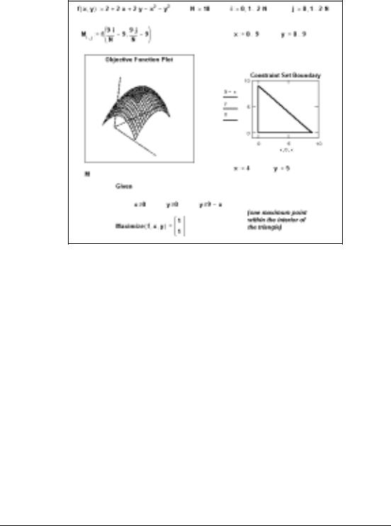
Comments There are five steps to solving a maximization problem:
1.Define the objective function f.
2.Provide an initial guess for all the unknowns you intend to solve for. This gives Mathcad a place to start searching for solutions.
3.Type the word given. This tells Mathcad that what follows is a system of equality or inequality constraints. You can type given or Given in any style. Just be sure you don't type it while in a text region.
4.Now type the equations and inequalities in any order below the word given. Use [Ctrl]= to type “ =.”
5.Finally, type the Maximize function with f and your list of unknowns. You can’t put numerical values in the list of unknowns; for example, Maximize(f, 2) isn’t permitted. Like given, you can type maximize or Maximize in any style.
The Maximize function returns values as follows:
•If there is one unknown, Maximize returns a scalar value that optimizes f.
•If there is more than one unknown, Maximize returns a vector of answers; for example, Maximize(f, var1, var2) returns a vector containing values of var1 and var2 that satisfy the constraints and optimize f.
The word Given, the equations and inequalities that follow, and the Maximize function form a solve block.
Functions |
63 |

By default, Mathcad examines your objective function and the constraints, and solves using an appropriate method. In Mathcad Professional, if you want to try different algorithms for testing and comparison, you can choose options from the context menu associated with Maximize (available via right mouse click), which include:
•AutoSelect − chooses an appropriate algorithm for you
•Linear option − indicates that the problem is linear (and thus applies linear programming methods to the problem) − guess values for var1, var2,... are immaterial (can all be zero)
•Nonlinear option − indicates that the problem is nonlinear (and thus applies these general
methods to the problem: the conjugate gradient solver; if that fails to converge, the Leven- berg-Marquadt solver; if that too fails, the quasi-Newton solver) − guess values for var1,
var2,... greatly affect the solution
•Quadratic option (appears only if the Mathcad Expert Solver product is installed) − indicates
that the problem is quadratic (and thus applies quadratic programming methods to the problem) − guess values for var1, var2,... are immaterial (can all be zero)
•Advanced options − applies only to the nonlinear conjugate gradient and the quasi-Newton solvers
These options provide more control for you to try different algorithms for testing and comparison. You may also adjust the values of the built-in variables CTOL and TOL. The constraint tolerance CTOL controls how closely a constraint must be met for a solution to be acceptable, e.g., if CTOL were 0.001, then a constraint such as x < 2 would be considered satisfied if the value of x satisfied x < 2.001. This can be defined or changed in the same way as the convergence tolerance TOL, which is discussed further in connection with the Find function. Since Maximize can be used without constraints, the value of CTOL will sometimes be irrelevant. Its default value is 0.
For an unconstrained maximization problem, the word Given and constraints are unnecessary.
Algorithm For the non-linear case: Levenberg-Marquardt, quasi-Newton, conjugate gradient For the linear case: simplex method with branch/bound techniques
(Press et al., 1992; Polak, 1997; Winston, 1994)
See also Find for more details about solve blocks; Minerr, Minimize
mean
Syntax |
mean(A) |
1 m – 1 |
|
|
|
||
Description |
Returns the arithmetic mean of the elements of A: mean(A) |
mn |
å |
= ------ |
|
||
Arguments |
|
|
i = 0 |
real or complex m × n matrix or vector |
|
|
|
A |
|
|
|
See also |
gmean, hmean, median, mode |
|
|
Statistics
n – 1
å Ai, j . j = 0
64 |
Chapter 1 Functions |
median
Syntax
Description
Arguments
A
See also
Statistics
median(A)
Returns the median of the elements of A. The median is the value above and below which there are an equal number of values. If A has an even number of elements, median is the arithmetic mean of the two central values.
real or complex m × n matrix or vector
gmean, hmean, mean, mode
medsmooth |
Regression and Smoothing |
Syntax medsmooth(vy, n)
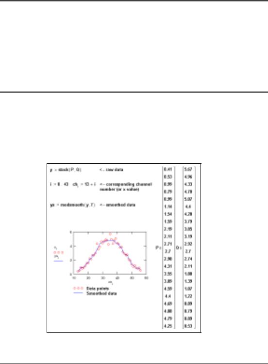
Description Creates a new vector, of the same size as vy, by smoothing vy with running medians.
Arguments
vy real vector
n odd integer, n > 0, the size of smoothing window
Example
Functions |
65 |

Comments Smoothing involves taking a set of y (and possibly x) values and returning a new set of y values that is smoother than the original set. Unlike the interpolation functions cspline, lspline, or pspline or regression functions regress or loess, smoothing results in a new set of y values, not a function that can be evaluated between the data points you specify. If you are interested in y values between the y values you specify, use an interpolation or regression function.
Whenever you use vectors in any of the functions described in this section, be sure that every element in the vector contains a data value. Because every element in a vector must have a value, Mathcad assigns 0 to any elements you have not explicitly assigned.
The medsmooth function is the most robust of Mathcad’s three smoothing functions because it is least likely to be affected by spurious data points. This function uses a running median smoother, computes the residuals, smooths the residuals the same way, and adds these two smoothed vectors together.
medsmooth performs these steps:
Algorithm
See also
1. |
Finds the running medians of the input vector vy. We'll call this vy′ . The ith element is |
|
|
given by: vy¢i = median(vyi – (n – |
1 ¤ 2), ¼, vyi, ¼, vyi + (n – 1 ¤ 2)) . |
2. |
Evaluates the residuals: vr = vy – |
vy¢ . |
3.Smooths the residual vector, vr, using the same procedure described in step 1, to create a smoothed residual vector, vr¢ .
4.Returns the sum of these two smoothed vectors: medsmooth(vy, n ) = vy¢ + vr¢ .
medsmooth will leave the first and last (n – 1 ) ¤ 2 points unchanged. In practice, the length of the smoothing window, n, should be small compared to the length of the data set.
Moving window median method (Lorczak)
ksmooth and supsmooth (alternative smoothing functions available in Mathcad Professional only)
mhyper |
(Professional) |
Special |
Syntax |
mhyper(a, b, x) |
|
Description |
Returns the value of the confluent hypergeometric function, 1F1(a;b;x ) or |
M(a;b ;x) . |
Arguments |
|
|
a, b, x |
real numbers |
|
Comments The confluent hypergeometric function is a solution of the differential equation:
d2 |
d |
and is also known as the Kummer function. |
|
x × -------y + (b – x ) × -----y – a × y= 0 |
|||
dx |
2 |
dx |
|
|
|
|
|
Many functions are special cases of this, e.g., elementary ones like |
|||
exp (x) |
= mhyper(1, 1, x) |
exp(x) × sin h(x) = x × mhyper(1, 2, 2 × x) |
|
and more complicated ones like Hermite functions.
Algorithm Series expansion, asymptotic approximations (Abramowitz and Stegun, 1972)
66 |
Chapter 1 Functions |
min |
Vector and Matrix |
Syntax |
min(A) |
Description |
Returns the smallest element in A. If A is complex, returns min(Re(A)) + i×min(Im(A)). |
Arguments |
real or complex m × n matrix or vector |
A |
|
See also |
max |
Minerr
Syntax
Description
Arguments
Solving
Minerr(var1, var2,...)
Returns values of var1, var2, ... which come closest to solving a prescribed system of equations, subject to prescribed inequalities. The number of arguments matches the number of unknowns. Output is a scalar if only one argument; otherwise it is a vector of answers.
var1, var2, ... real or complex variables; var1, var2, ... must be assigned guess values before using Minerr.
Example
Comments The Minerr function is very similar to Find and uses exactly the same algorithm. The difference is that even if a system has no solutions, Minerr will attempt to find values which come closest to solving the system. The Find function, on the other hand, will return an error message indicating that it could not find a solution. You use Minerr exactly the way you use Find.
Functions |
67 |

Algorithm
See also
Like Find, type the Minerr function with your list of unknowns. You can’t put numerical values in the list of unknowns; e.g., in the example above, Minerr(0.8, 1) isn’t permitted. Like Find, you can type Minerr or minerr in any style.
Minerr usually returns an answer that minimizes the errors in the constraints. However, Minerr cannot verify that its answers represent an absolute minimum for the errors in the constraints.
If you use Minerr in a solve block, you should always include additional checks on the reasonableness of the results. The built-in variable ERR gives the size of the error vector for the approximate solution. There is no built-in variable for determining the size of the error for individual solutions to the unknowns.
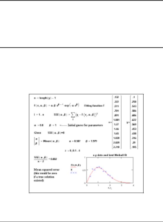
Minerr is particularly useful for solving certain nonlinear least-squares problems. In the example, Minerr is used to obtain the unknown parameters in a Weibull distribution. The function genfit is also useful for solving nonlinear least-squares problems.
In Mathcad Professional, the context menu (available via right mouse click) associated with Minerr contains the following options:
•AutoSelect − chooses an appropriate algorithm for you
•Linear option − not available for Minerr (since the objective function is quadratic, hence the problem can never be linear)
•Nonlinear option − indicates that the problem is nonlinear (and thus applies these general
methods to the problem: the conjugate gradient solver; if that fails to converge, the Leven- berg-Marquadt solver; if that too fails, the quasi-Newton solver) − guess values for var1,
var2,... greatly affect the solution
•Quadratic option (appears only if the Mathcad Expert Solver product is installed) − indicates
that the problem is quadratic (and thus applies quadratic programming methods to the problem) − guess values for var1, var2,... are immaterial (can all be zero)
•Advanced options − applies only to the nonlinear conjugate gradient and the quasi-Newton solvers
These options provide more control for you to try different algorithms for testing and comparison. You may also adjust the values of the built-in variables CTOL and TOL. The constraint tolerance CTOL controls how closely a constraint must be met for a solution to be acceptable, e.g., if CTOL were 0.001, then a constraint such as x < 2 would be considered satisfied if the value of x satisfied x < 2.001. This can be defined or changed in the same way as the convergence tolerance TOL. The default value for CTOL is 0.
For the non-linear case: Levenberg-Marquardt, quasi-Newton, conjugate gradient For the linear case: simplex method with branch/bound techniques
(Press et al., 1992; Polak, 1997; Winston, 1994)
Find for more details about solve blocks; Maximize, Minimize
68 |
Chapter 1 Functions |
Minimize
Syntax
Description
Arguments
Solving
Minimize(f, var1, var2,...)
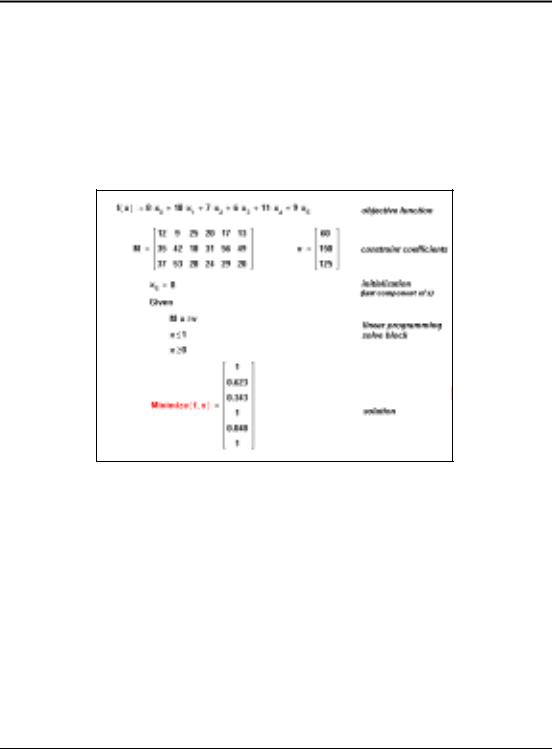
Returns values of var1, var2,... which solve a prescribed system of equations, subject to prescribed inequalities, and which make the function f take on its smallest value. The number of arguments matches the number of unknowns, plus one. Output is a scalar if only one unknown; otherwise it is a vector of answers.
f real-valued function
var1, var2, ... real or complex variables; var1, var2,.. must be assigned guess values before using Minimize.
Examples
Functions |
69 |
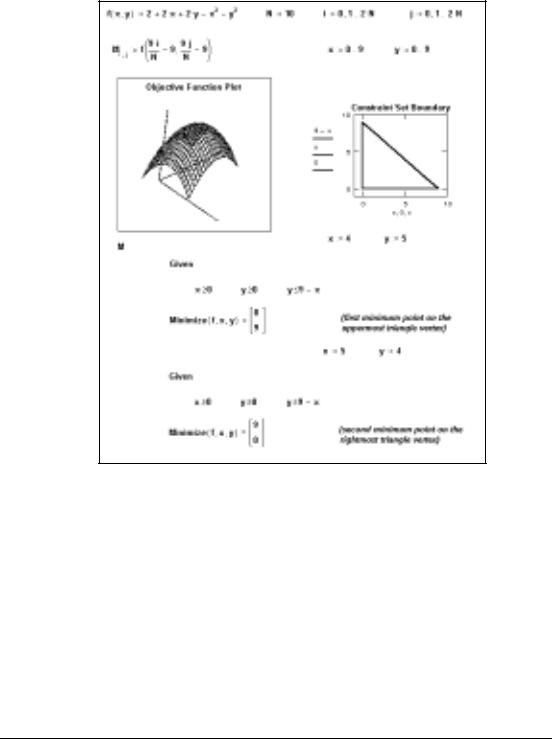
Comments There are five steps to solving a minimization problem:
1.Define the objective function f.
2.Provide an initial guess for all the unknowns you intend to solve for. This gives Mathcad a place to start searching for solutions.
3.Type the word given. This tells Mathcad that what follows is a system of equality or inequality constraints. You can type given or Given in any style. Just be sure you don't type it while in a text region.
4.Now type the equations and inequalities in any order below the word given. Use [Ctrl]= to type “ =.”
5.Finally, type the Minimize function with f and your list of unknowns. You can’t put numerical values in the list of unknowns; for example, Minimize(f, 2) isn’t permitted. Like given, you can type minimize or Minimize in any style.
70 |
Chapter 1 Functions |
