

CHAPTER 8
THE DEVELOPMENT OF GEOMETRY, II
PROJECTIVE GEOMETRY
THE LAWS OF PERSPECTIVE DRAWING—the technique used to portray three dimensions on a two dimensional surface—have been studied by artists since the Stone Age. For example, a fifteen thousand year old etching of a herd of reindeer on a bone fragment discovered by archaeologists creates the impression of distance by displaying the legs and antlers as if seen beyond the fully sketched animals of the foreground. The main perspective problem encountered by Egyptian artists was the portrayal of a single important object with the necessary dimension of depth: this was achieved in an ingenious manner by drawing a combination of horizontal and side view. Thus, for instance, in drawing a Pharaoh carrying a circular tray of sacrificial offerings, the top view of the tray is shown in half display by means of a semicircle, and on this half-tray is presented the sacrificial food as it would appear from above. This stylized method of expressing a third dimension persisted in Egyptian drawing for three thousand years. In America, an arresting method of achieving this effect was created by northwest Indian artists who, in their drawings of persons or animals, present views of both front and leftand right hand sides. The figures are drawn as if split down the back and flattened like a hide, with the result that each side of the head and body becomes a profile facing the other. Landscapes drawn by Chinese artists create the impression of space and distance by skillful arrangement of land, water and foliage. In drawing buildings, however, it was necessary to display the parallel horizontal lines of the construction, and for this the technique of isometric drawing was used. This is a simulation of perspective drawing in which parallel lines are drawn parallel, instead of converging as in true perspective.
In Europe, it was not until the first half of the fifteenth century that Italian painters, through the introduction of the horizon line and vanishing point, transformed perspective drawing into an exact science. The fundamental principles were worked out by the Florentine architect Filippo Brunelleschi (1377–1446) and developed by the painter Paolo Uccello (1397–1475). The formulation of the laws of perspective quickly transformed painting in Renaissance Italy, and the technique of perspective became an essential constituent in the works of later Italian masters. In his great wall-painting The
129

130 |
CHAPTER 8 |
Last Supper1, for example, Leonardo da Vinci (1542–1519) employs perspective in a subtle way to draw the viewer’s eye to the composition’s centre.
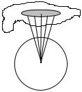
The origins of projective geometry lie in the study of perspective. A painter’s picture, or a photograph, can be regarded as a projection of the depicted scene onto the canvas or photographic film, with the painter’s eye or the focal point of the camera's lens acting as the centre of projection. For example, suppose we take a photograph of a straight railway track, with equally spaced ties, going directly away from us. In the photograph the parallel lines of the rails appear to converge, meeting at a vanishing point or “point at infinity”; the equal spaces between the ties appear as unequal; and the right angles between the rails and the ties appear as acute. A circular pond in the landscape would appear as an ellipse. Nevertheless the geometric structure of the original landscape can still be discerned in the photograph. This is possible only if the original scene and its image have certain geometric properties in common, properties which, unlike lengths and angles, are preserved under the passage from the one to the other. The object of projective geometry is to identify and investigate these properties in a general setting.
The transformation from scene to image may be described in the following way. Given any plane geometric figure (confining ourselves to plane figures for the sake of simplicity), let O be any point in the plane of the figure and imagine straight lines drawn from O to every point of the figure. Now allow this bundle of straight lines to be cut by any plane not passing through O. The resulting plane section of the lines through O yields a new figure in the cutting plane called the projection of the original figure. (In the case of our photograph, the original scene is the first figure, the photographic film is the cutting plane, and the focal point of the camera lens is the point O.) With each point or straight line of the original figure this process associates a definite point or straight line in the new figure; if a point P in the original figure lies on a straight line
l, in the new figure the associated point P′lies on the associated line l′. Any mapping of
one figure onto another by a projection of the kind we have just described, or the result of a finite sequence of such projections, is called a projective transformation. A projective transformation carries points into points and straight lines into straight lines in such a way as to preserve the incidence of points and lines. It does not preserve lengths or angles.
Two figures are homologous or projectively equivalent if each can be obtained from the other by a projective transformation. It is a fundamental fact of projective geometry that all the conic sections are projectively equivalent.
The set of all projective transformations furnishes another example of a group, since the result of successively performing any two of the operations in the set is still a transformation in the set; the set contains an identity transformation (“projection” onto the original plane); and each member of the set has an inverse whose composite with it in either order is the identity transformation (obtained by “reversing” the given projection). Projective geometry may be characterized completely as the study of those properties of figures which remain unchanged—are invariant—when acted upon by the elements of the group of projective transformations. Similarly, the set of all rigid
1 Happily, this masterpiece, in a sadly deteriorated state for as long as anyone can recall, has recently (1999) been restored.
THE DEVELOPMENT OF GEOMETRY, II |
131 |
motions in space forms a group: ordinary Euclidean geometry may then be identified as the geometry in which are studied those properties of figures, e.g., lengths and angles, which are invariant under the group of all such motions. As another example, the set of conformal (i.e., angle-preserving) transformations forms a group; conformal geometry
—which arose in connection with cartography, a science rich in geometric possibilities—is the study of properties of figures which are invariant under all the transformations in this group. These are all special instances of a general principle— enunciated by Klein in his Erlangen Program of 1872—which asserts that corresponding to every group of transformations in space there is a “geometry” comprising those properties of figures which are invariant under all the transformations in the given group. This principle establishes a systematic link between geometry and algebra, and enables geometries to be classified by the properties of their corresponding groups. Thus, for example, since the group of rigid motions may be identified as a subgroup of the group of conformal transformations, which is in turn a subgroup of the group of projective transformations, ordinary Euclidean geometry is implicitly contained in conformal geometry, which is in turn contained in projective geometry. Each of the first two geometries may accordingly be obtained by specialization from the more general geometry containing it.
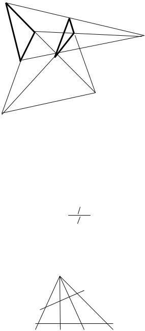
The first mathematician to take up the geometric problems suggested by perspective drawing was the Frenchman Girard Desargues (1591–1661) who was chiefly concerned to develop new methods for establishing properties of conics. In his major work on the subject, published in 1636, Desargues introduces, for each set of parallel lines, a ideal point—a point at infinity corresponding to the vanishing point of perspective drawing—which all the lines in the set have in common. He also introduces an ideal line—a line at infinity corresponding to the horizon line—and makes the assumption that all the new ideal points lie on that line. Thus in Desargues’ geometry each “ordinary” line contains exactly one “ideal” point—its “point at infinity”; each pair of lines meets at, or determines, a unique point; and each pair of points determines a unique line.
Desargues’ most famous result is his Triangle Theorem (see figure on following page).The theorem states: If two triangles ABC and A′B′C′ are situated in the same
plane so that the straight lines joining corresponding vertices are concurrent in a point O, then the corresponding sides, if extended, will intersect in three collinear points.
The two triangles ABC, A′B′C′ are said to be in perspective from O. This theorem
clearly belongs to projective geometry, since the whole figure can be projected onto any other plane without affecting any of the features mentioned in the theorem’s formulation. Its proof is based on this fact. For the points Q and R can then be
“projected to infinity”, causing the pairs of lines AB, A′B′and AC, A′C′ to meet at ideal points, so rendering each pair parallel. It is not difficult to show that, as a result, BC and B′C′ become parallel, so that their point of intersection P is now also an ideal
point. Thus under projection the points P, Q, and R all lie on the line at infinity, and are, accordingly, collinear. Projecting back to the original plane, P, Q, and R return to their original positions and remain collinear. So they must have been collinear in the first place. This proves the theorem.
132 |
CHAPTER 8 |
C
C′
B |
B′ |
O |
A A′
P
R
Q
As noted by Desargues, the theorem remains true—and is, surprisingly perhaps, more easily proved—in three dimensions, when the triangles lie in different, nonparallel planes.
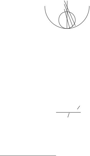
Desargues also established the fundamental fact that cross-ratio (a concept originally introduced by Pappus of Alexandria c.300 B.C.) is invariant under projection. The cross-ratio of four points A, B, C, D on a line l is defined to be the quantity
(ABCD) = CA CB DA DB
where a fixed direction on l is taken as positive. Referring to the figure below, Desargues proves that (ABCD) = (A′B′C′D′). Pappus had established this fact only when A and A′ coincide.
O
D
A B C
A′ |
B′ |
C′ |
D′ |
THE DEVELOPMENT OF GEOMETRY, II |
133 |
The next important contributor to projective geometry, Blaise Pascal (1623–1662) was at the same time a major literary figure and religious philosopher: his Pensées and Lettres Provinciales are classic works of French literature. Pascal is known for the famous theorem that bears his name: if a hexagon is inscribed in a conic, the three points of intersection of the pairs of opposite sides are collinear. Pascal did not supply an explicit proof of his theorem, but asserts that, since he knows it to be true for a circle, it must, by projection and section, be true of all conics.
During the latter half of the seventeenth century and throughout the eighteenth, coordinate geometry, with its quantitative and “analytic” methods, underwent rapid development. Projective geometry, on the other hand, with its emphasis on purely “synthetic” properties of geometric figures, remained becalmed. The stimulus that led to the revival of the subject in the nineteenth century was due in large measure to the French geometer Gaspard Monge (1746–1818), who, as an enthusiastic supporter of the French revolution, served as a technical advisor to Napoleon. In his Traité de Géométrie of 1799 Monge introduces the chief ideas of what was to become known as descriptive geometry, in which a three dimensional object is projected orthogonally onto two planes, one horizontal, the other vertical, so as to enable mathematical features of the object to be inferred.
The revival of projective geometry was carried out chiefly by Monge’s pupils
Charles-Julien Brianchon (1765–1864), Lazare M. N. Carnot (1753–1823), a major figure in the French revolution, and Jean-Victor Poncelet (1788–1867). Brianchon is remembered for the important theorem bearing his name: the three diagonals joining opposite vertices of a hexagon circumscribed about a conic are concurrent. Poncelet’s work of 1822, Traité des Propriétés Projectives des Figures, is really the first systematic work on projective geometry, in which the subject is treated as an independent discipline with methods and goals of its own. It was Poncelet who established projective geometry in its modern sense as the study of properties of figures which are invariant under projection.
Poncelet was also the first to recognize what later became known—through the work of Joseph-Diez Gergonne (1771–1859) and Jacob Steiner (1796–1863)—as the Principle of Duality. This is best illustrated by writing the statements of Pascal’s and Brianchon’s theorems side by side:
Pascal’s Theorem
If the vertices of a hexagon lie alternately on two straight lines, the points where opposite sides meet are collinear.
Brianchon’s Theorem
If the sides of a hexagon pass alternately through two points, the lines joining opposite vertices are concurrent.
Here we observe that each of these statements may be obtained from the other by interchanging terms such as “vertices” and “collinear” which make reference to points, with corresponding terms such as “sides” and “concurrent” which make reference to lines. The Principle of Duality is the assertion that the dual of any theorem of projective geometry is likewise a theorem of projective geometry. (Note, incidentally, that the dual of Desargues’ triangle theorem is precisely its converse!) The idea of duality, first discerned in projective geometry, has since been extended to other branches of mathematics, notably algebra.

134 |
CHAPTER 8 |
The advances made in projective geometry in the first part of the nineteenth century also excited the interest of geometers whose work was primarily in the algebraic spirit. From their efforts issued the subject of algebraic projective geometry. Here a leading idea is that of a homogeneous coordinate system. The first such system was introduced by the German mathematician August Ferdinand Möbius (1790–1868) in his work Der Barycentrische Calcul of 1827. Möbius’s idea was to start with a fixed triangle and to take as coordinates of any point P in the plane the amounts of mass which must be placed at each of the three vertices so as to make P the centre of mass or barycentre of the three masses (points lying outside the triangle being assigned some negative coordinates). Since multiplication of all three masses by the same nonzero constant does not change their barycentre, the coordinates are not unique, only their ratios being uniquely determined. Thus, as t varies over all nonzero real numbers, the triples (ta, tb, tc) all represent the same point, which justifies the use of the term “homogeneous” for the coordinate system.
The system of homogeneous coordinates normally employed by geometers today was invented by the German mathematician Julius Plücker (1801–1868). In his Analytisch-geometrische Entwickelungen of 1831, he takes the coordinates of any point P in the plane to be the signed distances (a, b, c) of P from the sides of a fixed triangle of reference. Since, again, the coordinates of a point can be multiplied by any nonzero constant without changing the point, Plücker went on to formulate what has become the standard definition of homogeneous coordinates in the plane, namely ordered triples (a, b, c) of real numbers not all zero, where the triples (ta, tb, tc) are taken to represent the same point as t varies over the nonzero real numbers. This is equivalent to replacing the usual rectangular coordinates (X, Y) by (x/t, y/t), so that the equations of curves become homogeneous in x, y, and t, that is, all terms have the same degree. In Plücker’s homogeneous coordinate system, ordinary points in the plane are represented by triples (a, b, c) with c ≠ 0, ideal points lying on ordinary lines by triples (a, b, 0) with a ≠ 0, and points (necessarily ideal) lying on the line at infinity by triples (0, b, 0) with b ≠ 0. The projective plane, one of the most important concepts in projective geometry, is defined to be the set of points determined in this way.
DIFFERENTIAL GEOMETRY.
The introduction of the methods of the calculus into coordinate geometry during the seventeenth century issued in a branch of mathematics now known as differential geometry2. In contrast with Euclidean or projective geometry, which is concerned with the whole of a diagram or a figure, that is to say, with its global properties, differential geometry concentrates on its local properties, that is, those arising in the immediate neighbourhoods of points of the figure, and which may vary from point to point. Thus, for example, one of the central concepts of differential geometry is the curvature of a
2 The term “differential geometry” was introduced in 1894 by the Italian mathematician Luigi Bianchi (1856– 1928).
THE DEVELOPMENT OF GEOMETRY, II |
135 |
(plane) curve at a point, which is a quantity measuring the “sharpness of bending” of the curve in the neighbourhood of the point. More suggestively, if we think of the curve as being traced out by a moving particle, then the curvature at a given point is (proportional to) the rate at which the object’s path is changing direction at that point. The curvature of a straight line at any point on it is then zero, as is, more generally, that at a point of inflection of any curve, while that of a circle is constantly equal to the reciprocal of the length of its radius. This latter fact suggests that we define the radius of curvature of a curve C at a point P to be the reciprocal of the curvature at P. The radius of curvature is then the radius of the so-called osculating, or “kissing”, circle—
n |
C |
P
a term first introduced by Leibniz—to the curve at P. This circle is the one which approximates best to the curve at P; its centre is called the centre of curvature of C at
P.
Many of the basic concepts of differential geometry were introduced by Christiaan Huygens (1629–1675) in his Horologium Oscillatorium of 1673, a work largely devoted, as its title suggests, to the theoretical design of accurate pendulum clocks. Huygens obtained his results by means of purely geometrical methods and it was in fact Newton who, in his Geometria Analytica of 1736, first employs the methods of the calculus in this area, obtaining results essentially identical to those of Huygens. Thus, for example, both Huygens and Newton show that the centre of curvature of a curve at a point P on it is the limiting position of the point of intersection of a fixed normal3 n to a curve at P with an adjacent normal moving toward n, as in the figure above. They both show that the radius of curvature of the curve at the point (x, y) is, using the notation of the calculus,
[1+(dy dx)2 ]32
d2 y dx2
The first steps in three-dimensional differential geometry were taken by Clairault in his Recherche sur les Courbes à Double Courbure of 1731, a work treating of both curves and surfaces. Clairault termed space curves “curves of double curvature” because he recognized that the projection of a space curve onto each of two perpendicular planes would give rise to a pair of curves each possessing an
3 A normal to a curve at a point P on it is a straight line passing through P perpendicular to the tangent to the curve at P.
136 |
CHAPTER 8 |
independent curvature. He also saw that a space curve can have an infinity of normals in a plane perpendicular to the tangent at a point.
The next important advances in the theory of space curves were made in 1774 and 1775 by Leonhard Euler (1707–1783). He introduces the concept of osculating plane to a space curve at a point on it, that is, the plane lying closest to the curve in the neighbourhood of the point. Both the tangent and the osculating circle to the curve at the point lie in this plane. Euler defines the curvature of the curve at the point to be the reciprocal of the length of the radius of the osculating circle to the curve at the point.
In 1806 Michel-Ange Lancret (1774–1807), a student of Monge, introduced the scheme, now known as the moving trihedron, by means of which space curves are analyzed today. Lancret singled out three principal directions at each point P of a space
|
b |
n |
t |
C
P
curve C: the tangent t, the normal n in the osculating plane, and the common perpendicular to these, the binormal b. It is helpful to think of these as constituting a rigid frame of rectangular axes, with P as origin, moving forward and rotating as P traverses the curve with unit speed. The angular velocity of the frame about the binormal is then the curvature at P. The angular velocity of the frame about the tangent —the torsion of the curve at P—represents the rate at which the curve deviates from a plane at the point. The significance of the curvature and torsion of a curve is that together they provide a complete description of the curve: if we are given both at each point of the curve, then the curve is uniquely determined except for spatial position. This fact became clear when the theory of space curves was brought into essentially its
modern form by Augustin-Louis Cauchy (1789–1857) in his Leçons sur les Applications du Calcul Infinitésimal à la Géométrie of 1826.
The Theory of Surfaces
The origins of the differential geometry of surfaces began in the seventeenth century with the study of geodesics, that is, curves of least length on a surface (initially, in accordance with the needs of navigation, that of the earth). In 1697 Jean Bernoulli (1667–1748) posed the problem of finding the shortest curve joining two points on a convex surface, and in 1698 observed that the osculating plane at any point of such a curve on a surface is normal to the surface at that point. Also in 1698 Jacques Bernoulli (1655–1705 ) determined the geodesics on cylinders, cones, and surfaces of revolution.
THE DEVELOPMENT OF GEOMETRY, II |
137 |
The general form of the equations for geodesics on surfaces was obtained by Euler in 1728.
The theory of surfaces was placed on a sound basis by Euler in his Recherches sur la Courbure des Surfaces of 1760. In this work he introduces the principal curvatures of a surface at a point. These are defined as follows. Given a surface S and a point P on it, the assemblage of planes through a normal n to S at P cuts S in a family of plane curves, each of which has a curvature at P. The two planes containing the curves with the largest and smallest curvatures can then be shown to be perpendicular to each other (assuming they are distinct). These two curvatures are then the principal curvatures of the surface S at P. It was shown in 1776 by Jean-Baptiste Meunier (1754–1793) that the only surfaces for which the two principal curvatures everywhere coincide are planes or spheres.
Euler was the first to study developable surfaces, that is, surfaces which can be flattened out onto a plane without distortion. This study had its origins in cartography, whose practitioners had come to recognize the awkward fact that a sphere cannot be cut and so flattened, thus making the task of mapping the earth’s surface a subtle one. In his work De Solidus quorum Superficium in Planum Explicare Licet of 1771, Euler formulates necessary and sufficient conditions for a surface to be developable, and proves the striking result that the family of tangents to a space curve constitutes a developable surface.
In 1827 Gauss published his definitive paper on surfaces, Disquisitiones Generales circa Superficies Curvas, in which the study of the curvature of surfaces is raised to a new level. Gauss introduces a new measure of curvature, the total or Gaussian curvature, of a surface. To define Gaussian curvature, we consider a small region R on a surface S, and at each point of R we erect a normal to S. These normals
R
S
 A
A
B
will form a cone, or solid angle, whose size is measured by the area of the region A in which a sphere B of unit radius intersects it. This size will depend both on the area of R and, crucially, on the extent to which it is curved. Thus the curvature of R may be characterized as the ratio of the size of the solid angle to the area of R. The total or Gaussian curvature of S at P is then defined to be the limit of this ratio as R shrinks to the point P.
Gauss proved that the total curvature of a surface at a point is the product of Euler’s principal curvatures at that point. More significantly still, he established the following remarkable property of total curvature. Suppose that the surface has been stamped out from some flexible but inextensible material, a thin sheet of tin, for example, so that it
138 |
CHAPTER 8 |
can be bent into various shapes without stretching or tearing it. During this process the principal curvatures will change but, as was shown by Gauss, their product, and hence the total curvature, will remain unchanged at every point. This shows that two surfaces with different Gaussian curvatures are intrinsically distinct, the distinction consisting in the fact that the surfaces can never be deformed without stretching or tearing in such a way as to enable them to be superposed on one another. Thus, for example, a segment of the surface of a sphere can never be distorted in this manner so as to lie flat on a plane or on a sphere of different radius. Total curvature accordingly furnishes a measure of the curvature of a surface which is intrinsic, that is, not dependent on the fact that the surface is part of three-dimensional space. The idea that surfaces have intrinsic geometries was to serve as the basis for Riemann’s far-reaching generalization of geometry, to which we now turn.
Riemann’s Conception of Geometry
In his famous lecture of 1854, published as a paper in 1868, “On the Hypotheses which Lie at the Foundations of Geometry,” Riemann introduces the idea of an intrinsic geometry for an arbitrary “space” which he terms a multiply extended manifold. Riemann conceives of a manifold as being the domain over which varies what he terms a multiply extended magnitude. Such a magnitude M is called n-fold extended, and the associated manifold n-dimensional, if n quantities—called coordinates—need to be specified in order to fix the value of M. For example, the position of a rigid body is a 6- fold extended magnitude because three quantities are required to specify its location and another three to specify its orientation in space. Similarly, the fact that pure musical tones are determined by giving intensity and pitch show these to be 2-fold extended magnitudes. In both of these cases the associated manifold is continuous in so far as each magnitude is capable of varying continuously with no “gaps”. By contrast, Riemann terms discrete a manifold whose associated magnitude jumps discontinuously from one value to another, such as, for example, the number of leaves on the branches of a tree. Of discrete manifolds Riemann remarks:
Concepts whose modes of determination form a discrete manifold are so numerous, that for things arbitrarily given there can always be found a concept…under which they are comprehended, and mathematicians have been able therefore in the doctrine of discrete quantities to set out without scruple from the postulate that given things are to be considered as being all of one kind. On the other hand there are in common life only such infrequent occasions to form concepts whose modes of determination form a continuous manifold, that the positions of objects of sense, and the colours, are probably the only simple notions whose modes of determination form a continuous manifold. More frequent occasion for the birth and development of these notions is first found in higher mathematics.
The size of parts of discrete manifolds can be compared, says Riemann, by straightforward counting, and the matter ends there. In the case of continuous manifolds, on the other hand, such comparisons must be made by measurement. Measurement, however, involves superposition, and consequently requires the positing of some magnitude—not a pure number—independent of its place in the manifold. Moreover, in a continuous manifold, as we pass from one element to another in a
THE DEVELOPMENT OF GEOMETRY, II |
139 |
necessarily continuous manner, the series of intermediate terms passed through itself forms a one-dimensional manifold. If this whole manifold is now induced to pass over into another, each of its elements passes through a one-dimensional manifold, so generating a two-dimensional manifold. Iterating this procedure yields n-dimensional manifolds for an arbitrary integer n. Inversely, a manifold of n dimensions can be analyzed into one of one dimension and one of n – 1 dimensions. Repeating this process finally resolves the position of an element into n magnitudes. These ideas are not dissimilar to those put forward by Grassmann in his Ausdehnungslehre.
Riemann thinks of a continuous manifold as a generalization of the threedimensional space of experience, and refers to the coordinates of the associated continuous magnitudes as points. He was convinced that our acquaintance with physical space arises only locally, that is, through the experience of phenomena arising in our immediate neighbourhood. Thus it was natural for him to look to differential geometry to provide a suitable language in which to develop his conceptions. In particular, the distance between two points in a manifold is defined in the first instance only between points which are at infinitesimal distance from one another. This distance is calculated according to a natural generalization of the distance formula in Euclidean space. In n-dimensional Euclidean space, we recall that the distance ε between two points P and Q with coordinates (x1 ,…, xn) and (x1 + ε1,…, xn + εn) is given by
ε2 = ε2 |
+...+ε2 . |
(1) |
1 |
n |
|
In an n-dimensional manifold, the distance between the points P and Q—assuming that the quantities εi are infinitesimally small—is given by Riemann as the following generalization of (1):
ε2 = ∑ gij εi εj ,
where the gij are functions of the coordinates x1 ,…, xn, gij = gji and the sum on the right side, taken over all i, j such that 1 ≤ i, j ≤ n, is always positive. The array of
functions gij is called the metric of the manifold. In allowing the gij to be functions of the coordinates Riemann allows for the possibility that the nature of the manifold or “space” may vary from point to point, just as the curvature of a surface may so vary.
Riemann also extends Gauss’s concept of total curvature of a surface to manifolds. In doing so his goal was to characterize Euclidean space, and, more generally, spaces which are homogeneous in that within them figures can be moved about without change of size or shape. Like total curvature of a surface, Riemann’s notion of curvature of a manifold is an intrinsic property of the manifold (or, more precisely, of its metric); it is not required to think of the manifold as being situated in some manifold of higher dimension. Riemann introduces manifolds of constant curvature: by definition, in these spaces all measures of curvature are equal and remain unchanged from point to point, so yielding the required homogeneity property. In his paper Riemann states, but does not prove, that in a manifold of constant curvature the metric is given by

140 CHAPTER 8
|
|
|
|
∑ε2 |
|
||
ε2 = |
|
|
|
|
i |
. |
|
1 |
+ 1 |
4 |
α∑ x2 |
||||
|
|
||||||
|
|
|
|
i |
|
||
Riemann observes that when α is positive we obtain a spherical space, when α = 0, a Euclidean (flat) space, and when α is negative, a surface resembling the inside of a torus.
In the final section of his paper, Riemann applies his ideas to the problem of determining the structure of physical space. He points out that, as regards physical space, infinitude must be carefully distinguished from boundlessness. For example, the surface of a sphere is finite but unbounded and, for all we know, the same may be true of physical space. In any case it is the boundlessness, rather than the infinitude of space that is required for maneuvering in the external world, so that the former has a far greater empirical certainty than the latter. Moreover, if space has a constant positive measure of curvature, however small, then it would take the form of a spherical surface and would accordingly be finite and boundless.
Riemann concludes his discussion with the following words, the last sentence of which proved to be prophetic:
While in a discrete manifold the principle of metric relations is implicit in the notion of this manifold, it must come from somewhere else in the case of a continuous manifold. Either then the actual things forming the groundwork of a space must constitute a discrete manifold, or else the basis of metric relations must be sought for outside that actuality, in colligating forces that operate on it. A decision on these questions can only be found by starting from the structure of phenomena that has been confirmed in experience hitherto…and by modifying the structure gradually under the compulsion of facts which it cannot explain…This path leads out into the domain of another science, into the realm of physics.
Riemann is saying, in other words, that if physical space is a continuous manifold, then its geometry cannot be derived a priori—as claimed, famously, by Kant—but can only be determined by experience. In particular, and again in opposition to Kant, who held that the axioms of Euclidean geometry were necessarily and exactly true of our conception of space, these axioms may have no more than approximate truth.
Riemann’s final sentence proved to be prophetic because in 1916 his geometry— Riemannian geometry—was to provide the basis for a landmark development in physics, Einstein’s celebrated General Theory of Relativity. In Einstein’s theory, the geometry of space is determined by the gravitational influence of the matter contained in it, thus perfectly realizing Riemann’s contention that this geometry must come from “somewhere else”, to wit, from physics.
TOPOLOGY
Combinatorial Topology
The set of all continuous (reversible) transformations in space, i.e., deformations of figures or objects which occur without tearing anything apart, also forms a group, and the corresponding “geometry” is called topology (from Greek topos, “place”). By what

THE DEVELOPMENT OF GEOMETRY, II |
141 |
we have already said, topology must then involve the consideration of properties of figures which are invariant under any continuous transformation. Calling two figures topologically equivalent if each one can be continuously and reversibly deformed into the other, we say that a property of a figure is topological if, when possessed by a given figure, it is also possessed by all figures topologically equivalent to the given one. Topology may now be broadly defined as the study of topological properties.4 We see immediately that, in general, projective properties such as, e.g., being a triangle or a straight line are not topological, since a triangle is evidently topologically equivalent to any simple closed curve and a straight line to any open curve. (To see this, imagine both triangle and line made from cooked pasta or modelling clay.) Topological properties are grosser than projective ones, since they must stand up under arbitrary continuous deformations. So, for example, a topological property of the triangle is not its triangularity but the property of dividing the plane into two—“inside” or “outside”— regions, as well as the property that, if two points are removed, it falls into two pieces, while if only a single point is removed, one piece remains. As another example we may consider the properties of one-sidedness or two-sidedness of a surface. The standard one-sided surface—the so-called Möbius strip (or band), discovered independently in 1858 by Möbius and J. B. Listing5 (1806–1882)—may be constructed by gluing together the two ends of a strip of paper after giving one of the ends a half twist. Both oneand two-sidedness are topological properties.
The historical record shows that the first theorem of an indisputably topological nature is that proved by Euler6 in 1752. This is the assertion that, for any simple polyhedron (i.e., closed, convex, and without holes), the numbers v of vertices, e of edges and f of faces are related by the equation
v – e + f = 2. |
(1) |
Here is a proof of this assertion, based on that given by Cauchy in 1811. Imagine the given simple polyhedron to be hollow and made of thin rubber. Now cut out one of its faces and deform the remaining surface so as to stretch it out flat on a plane. In this way the network of vertices and edges of the original polyhedron is flattened out into a similar network on the plane, without changing the number of either. However, the number of polygons in the plane is one less than in the original polyhedron, since one face has been removed. We show that, for the plane network, v – e + f = 1, so that, when the excised face is counted, v – e + f = 2 for the original polyhedron.
4In view of the fact that a doughnut and a coffee cup (with a handle) are topologically equivalent, John Kelley famously defined a topologist to be someone who cannot tell the two apart. On this light-hearted note, the published phrase containing the maximum number of references to topology and geometry must surely be
On the analytic and algebraic topology of locally Euclidean metrization of infinitely differentiable Riemannian manifolds,
part of a line in Tom Lehrer’s wittily irreverent “mathematical” song Lobachevsky.
5 It was also Listing who, in his work Vorstudien zur Topologie of 1848, first uses the term “topology”; the subject being known prior to this as analysis situs, “positional analysis”.
6The content of the theorem appears already to have been known to Descartes a century earlier.

142 |
CHAPTER 8 |
First, we convert the plane network into a number of linked triangles by drawing all the diagonals in polygons which are not already triangles. This does not affect the value of v – e + f, because each time a diagonal is drawn, the values of e and f are both increased by 1, while that of v is unaffected. Next, from any triangle lying on the boundary of the network we remove that portion which does not belong to any other triangle. Any such triangle has either one or two edges on the boundary. In the first case, just the outer edge and the face of the triangle are removed, so that e and f are both decreased by 1, while v is unchanged, and accordingly v – e + f remains the same. In the second case, the face, the two outer edges and one vertex of the triangle are removed, so that v and f are both diminished by 1, and e by 2, again leaving v – e + f unaffected. Continuing in this way we can remove triangles on the boundary (which of course changes each time a triangle is removed) until finally only a single triangle remains, with its three edges, three vertices, and one face. For this simple network, v – e + f clearly has value 1. Since the procedure of erasing triangles has not altered the value of v – e + f, this quantity must have value 1 for the original plane network, and hence also for the polyhedron with one face missing. So v – e + f = 2 for the original polyhedron, as claimed.
The topological nature of Euler’s relationship (although Euler himself failed to recognize it) may be discerned through the fact that equation (1) will continue to hold when the polyhedron is subjected to an arbitrary continuous deformation. Under such a deformation, the edges will, in general, cease to be straight, and the faces cease to be flat, but, nevertheless, they will remain edges and faces. Thus the deformation will preserve both the number of edges and the number of faces, as well as, of course, the number of vertices, so that the relationship above will remain valid, even though the procedure will cause the surface of the polyhedron to become curved . The vertices, edges and faces of the original polyhedron may be considered to constitute a map drawn on the resulting (curved) surface. When all the faces of the map so constituted are triangles—curved or rectilinear—it is known as a triangulation of the surface. As we saw in the proof of Euler’s theorem, the number v - e + f for an arbitrary map is the same as for the triangulation obtained from it by drawing all the diagonals in its faces. Accordingly, as far as the value of v - e + f is concerned, we lose nothing by confining our attention to triangulations. This fact is the basis of the combinatorial method in topology, in which the properties of the surface are investigated by means of one of its triangulations7. Of course, for this purpose one only considers properties of the triangulation which are independent of its particular identity and thus, being common to all triangulations of the given surface, express some property of the surface itself.
Euler's relationship (1) in fact yields one such property. Let us call the expression v - e + f, where v, e, and f are, respectively, the number of vertices, edges and triangles of the given triangulation its Euler characteristic. Then Euler's theorem can be taken as asserting that for all triangulations of a surface topologically equivalent to a sphere the Euler characteristic is two. As it turns out, all triangulations of any given surface have the same Euler characteristic, which we call the Euler characteristic of the given
7This is an instance of the reduction of the continuous (in this case, a surface) to the discrete (in this case, the finite configuration provided by a triangulation). See Chapter 10.
THE DEVELOPMENT OF GEOMETRY, II |
143 |
surface. This number is a topological invariant in the sense that its value is the same for all topologically equivalent surfaces. For example, the Euler characteristic of a cylinder or a torus (doughnut) is zero, and that of a figure eight shaped pretzel is –2. In general, the Euler characteristic of a surface with k “holes” is 2 – 2k.
Another famous problem whose topological nature came later to be recognized is the Königsberg Bridge Problem. Königsberg lies on the banks of the river Pregel, which contains two islands linked to each other and to the banks in the following way:
C
A
 B
B
D
For many years the residents of Königsberg had tried without success to find a way of crossing all seven bridges exactly once on a continuous walk. Euler got wind of the problem and, in 1735, solved it in the negative. He achieved this by simplifying the formulation of the problem, replacing the land by points A, B, C, D and the linking bridges by arcs or lines as in the figure:
C
A B
D
The entire configuration is called a graph; its points are called vertices, and its lines and arcs edges. The problem of crossing the bridges is thus reduced to that of traversing the graph in one continuous sweep of the pencil without lifting it from the paper. Calling a vertex odd or even according as the number of edges leading from it is odd or even, Euler discovered that a graph can be continuously traversed in the manner specified if all its vertices are even. If the graph contains at least one, but no more than two odd vertices, it can be traversed in one journey, but it is not possible to return to the starting point. In general, if the graph contains 2n odd vertices, it will require exactly n journeys to traverse it. In the case of the Königsberg bridges n = 2.
It was Möbius who gave topology its first explicit formulation. In his Theory of Elementary Relationships of 1863 he proposed studying the relationship between two figures whose points can be placed in biunique correspondence in such a way that neighbouring points correspond to neighbouring points, that is, continuously. It is in this work that the technique of triangulation is first employed in a systematic way and used to show that any polyhedron may be systematically reduced to an assemblage of
144 |
CHAPTER 8 |
triangles. Möbius also showed that certain curved surfaces could be dissected and displayed as polygons with sides properly identified. Thus, for example, a double torus can be represented as the polygon below, where edges marked alike are to be identified:
*
H H
*
Another example of a topological property derives from the so-called four-colour theorem—first suggested by Möbius in 1840—which states that any map in the above sense drawn on the surface of a sphere (or a plane) can be coloured with at most four colours, in such a way that any two regions with a common boundary line are assigned different colours. The simplest map in the plane requiring four colours looks like this:
The problem of proving that four colours suffice for any map has an entertaining, if comparatively brief history, and includes what is probably the most infamous fallacious “proof” in the whole of mathematics. This was announced in 1879 by A. B. Kempe and for more than a decade was believed to be sound until P. J. Heawood spotted the flaw in 1890. By revising Kempe's proof Heawood was, however, able to establish that five colours are sufficient. In 1976, W. Haken and K. Appel finally established that four are enough, but only by resorting to the use of a computer program to check several hundred basic maps. It is with a certain reluctance that mathematicians have come to accept this “proof”, since it cannot be examined in the traditional line-by-line manner that has always been taken for granted. The question of the legitimacy of “computer proofs” in mathematics has sparked a lively debate in recent years.
A major stimulus to the development of topology resulted from Riemann’s work in the theory of functions of a complex variable in the middle decades of the nineteenth century. He introduced the concept of connectivity of a surface, defining it in the following way:
THE DEVELOPMENT OF GEOMETRY, II |
145 |
If upon a surface there can be drawn n closed curves which neither individually nor in combination completely bound a part of the surface, but with whose aid every other closed curve forms the complete boundary of a part of the surface, then the surface is said to be (n + 1)-fold connected.
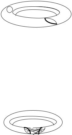
Riemann observes that the connectivity of a surface can be reduced by cutting it, giving as an example the torus, which is triply connected but can be reduced to a singly, or simply connected surface by means of one latitudinal and one longitudinal cut:
Riemann recognized that connectivity is a topological property and that it could be used to classify surfaces. In the latter half of the nineteenth century the term genus was introduced in connection with this classification. The genus of a surface is the largest number of nonintersecting simple closed curves that can be drawn on the surface without separating it: thus a sphere has genus 0, a torus genus 1 and, in general, a surface with p holes genus p. Riemann regarded it as intuitively evident that topologically equivalent surfaces have the same genus and observed that surfaces of genus 0 are topologically equivalent, each being mappable onto the surface of a sphere.
In 1882 Klein suggested a topological model for a surface of genus p which has become standard, namely, a sphere with p “handles” attached. It is clear that a closed surface of genus p can be continuously deformed into such an object, and so is topologically equivalent to it. Using this model it is quite easy to show that the Euler characteristic of a surface S of genus p is 2 – 2p. For S may be taken to be a sphere with p handles, and each handle is attached to the sphere at two bounding curves. Cut the sphere along one of these bounding curves for each handle, and straighten the handles out. Each handle will now have a free edge bounded by a new curve having the same number of edges and vertices. Thus the additional edges and vertices exactly counterbalance one another, and so, since no new faces have been created, the Euler characteristic remains unchanged. Now flatten out the protruding handles, so that the resulting surface is simply a sphere from which 2p regions have been removed. Since the Euler characteristic of a sphere is 2, that of a sphere with 2p holes is clearly 2 – 2p, hence also for the sphere with p handles, and any surface of genus p.
The problem of the topological equivalence of closed surfaces was investigated intensively throughout the latter half of the nineteenth century. In 1874 a major advance was made by Klein, who showed that two orientable closed surfaces of the same genus are topologically equivalent. Here by an orientable surface is meant one equipped with a triangulation whose constituent triangles can be oriented in such a way that any side common to two triangles has opposite orientations induced on it. Thus any
146 |
CHAPTER 8 |
two-sided surface such as a sphere or a plane is orientable, but a one-sided surface such as a Möbius strip is not.
By the end of the nineteenth century the only area of topology to have been more or less worked out was the topology of closed surfaces. Beginning in 1895 Poincaré began to develop the topological theory of spaces more general than surfaces, thereby establishing combinatorial topology as an autonomous branch of mathematics. In this general theory, later elaborated by the Dutch mathematician L. E. J. Brouwer (1882– 1966), triangles are replaced by higher-dimensional objects known as simplexes—a one-dimensional simplex is a line segment, a two-dimensional simplex a triangle, a three-dimensional simplex a tetrahedron, and an n-dimensional simplex a generalized tetrahedron with n + 1 vertices. The role of triangulations is assumed by complexes, where a complex is defined to be an assemblage K of simplexes any two of which meet, if at all, in a common face, and every face of a simplex in K is also in K. Using these ideas the concept of connectivity and the Euler characteristic can be extended to spaces of higher dimensions.
Another important idea introduced by Poincaré is the so-called fundamental group of a space, the initial concept of what was to evolve into the subject known today as algebraic topology. The idea arises from considering the distinction between simply and multiply connected plane regions. In the interior of a circle, for instance, every closed curve can be contracted to a point, while in an annulus or circular ring a closed curve enclosing the inner circular boundary cannot be so contracted. Now consider an arbitrary region R in the plane—which we take as a typical “space”— and the closed curves that begin and end at a given point x0 of R. Curves such as c and d in the figure below which can be continuously deformed into one another while remaining entirely within R are called homotopic and are considered to form one class. Roughly speaking,
e
x0 c
d
R
a class in this sense—a homotopy class—comprises those curves going round the same holes the same number of times. Thus the closed curves starting and ending at x0 and not enclosing any holes form one homotopy class, while those such e enclosing the two upper holes will form another. Two curves can be “merged” into the curve obtained by traversing first the one and then the other. This gives rise to an operation of multiplication on homotopy classes: the product of two homotopy classes C, D is to consist of all the curves obtained by merging a member of C with a member of D (in the order specified). It can now be shown that with this operation the collection of all homotopy classes forms a group, known as the fundamental group of the space R with base point x0. Usually the structure of the fundamental group is independent of the choice of base point, and the group is simply called the fundamental group of the space in question. In this way an algebraic structure—a group—is associated with each space.
THE DEVELOPMENT OF GEOMETRY, II |
147 |
The properties of the fundamental group reflect the connectivity of the space. Any simply connected space has a trivial fundamental group consisting of just the identity element, while the fundamental group of an annular region in the plane is isomorphic to the additive group of integers.
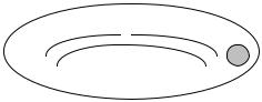
A further concept of algebraic topology which can be traced back to Poincaré is that of a homology group, a somewhat different device for charting the connectivity properties of the space. To explain the idea, consider the difference between the surface of a torus T and that of a sphere. It is intuitively obvious that any closed curve on the sphere cuts the surface into two separate regions. But this is not true in the case of the torus:
 B
B
Z
For cutting along the curve Z here does not disconnect the torus, which means that Z is not the boundary of a portion of T. But of course there are closed curves such as B which are boundaries.
Because the intuitive idea of a closed curve involves the notion that it “goes around something”, a closed curve such as B or Z is called a cycle on T. While B and Z are simple curves, i.e., do not cross themselves, we do not insist that all cycles be simple in this sense. The special cycles such as B—the bounding cycles—do not tell us very much about the structure of T, so for the moment we ignore them. It is the nonbounding cycles such as Z which are of interest.
Obviously there are infinitely many nonbounding cycles on the torus. But we shall see that these admit a simple description. First, the two cycles Z1 and Z2 in the figure on the page following are not intrinsically different since they both go round the torus once latitudinally. More significantly, however, taken together they form
Z1 Z2
the boundary of a portion of the torus, e.g. the shaded cylinder. The idea of taking cycles together suggests that they can be “added”. So let us extend our definition of cycle to include all unions of finitely many closed curves. Thus the operation of union gives a well-defined sum of two cycles, and we see that the sum Z1 + Z2 of the two
148 |
CHAPTER 8 |
cycles considered above is a bounding cycle. This leads to the idea of calling two cycles Z and Z′ homologous if Z + Z′ is a bounding cycle. This relation partitions
cycles into mutually disjoint classes—the homology classes. The purely latitudinal cycles such as Z form one such homology class, the purely longitudinal ones another, and the bounding cycles still another. It is not difficult to show that every nonbounding cycle is homologous to a sum of a purely latitudinal cycle and a purely longitudinal one.
Now we can define an operation of addition on homology classes by stipulating that the sum of two such classes is to be the class consisting of the cycles obtained by adding a cycle of the first class to one of the second. With this operation the set of homology classes becomes a group—the homology group of the torus. It has 4 elements, namely the homology classes O, A, B, C consisting respectively of bounding cycles, purely latitudinal cycles, purely longitudinal cycles, and sums of cycles from A and B. It has neutral element O, and its addition table is:
A + A = B + B = C + C = O
A + B = B + A = C, A + C = C + A = B, B + C = C + B = A.
In a natural sense the two elements A and B may be said to generate the homology group of the torus; this corresponds to the fact that the torus has two “holes” around which curves can curves can go latitudinally or logitudinally. Topologists express this by saying that the Betti number—named after the Italian mathematician Enrico Betti (1823–1892)—of the torus is 2.
Using the notions of simplex and complex already mentioned, homology groups can be constructed for each space. The number of generators of this group—the Betti number of the space—is the number of “holes” in the space. Both homology and fundamental groups thus reflect the connectivity of the space. In general, homology groups are considerably easier to determine than fundamental groups. But the latter are more sensitive, as can be seen by considering the surface—depicted below—obtained from a torus by removing an open disc D. While the fundamental group of this surface is clearly different from that of the torus, the homology group remains unchanged: the new “hole” is invisible as far as the latter is concerned.
 D
D
To conclude our account of combinatorial topology, we mention its most outstanding open problem, the so-called Poincaré conjecture. In 1904 Poincaré conjectured that every simply connected, closed orientable three-dimensional space is topologically equivalent to the three-dimensional sphere. Informally, the conjecture
THE DEVELOPMENT OF GEOMETRY, II |
149 |
says that the three-dimensional sphere is the only possible type of bounded threedimensional space containing no holes. This famous claim remains unresolved.
Remarkably, however, the corresponding assertion for dimensions ≥ 4 has been established.
Point-set Topology
The key feature which distinguishes topology from other branches of geometry is its concern with continuity, a notion which in turn involves the idea of proximity. Thus a continuous function is, intuitively, one which does not pull “neighbouring” points of its domain “too far” apart. But what exactly do these terms mean? In the first decades of the twentieth century the use of set theory in developing point-set or general topology enabled these concepts to be rigorously defined, thereby placing the whole subject of topology on a solid basis.
The central concept of point-set topology is that of topological space. This concept may be defined in a variety of equivalent ways; the one given here—due originally to Felix Hausdorff (1868–1942)—is framed in terms of the concept of neighbourhood.
Suppose we are given a set X of elements which may be such entities as points in n- dimensional space, plane or space curves, complex numbers or quaternions, although we make no assumptions as to their exact nature. The members of X will be called points. Now suppose in addition that corresponding to each point x of X we are given a collection Nx of subsets of X, which we call the neighbourhoods of x, subject to the following conditions:
(i)each member of Nx contains x;
(ii)the intersection of any pair of members of Nx includes a member of Nx;
(iii)for any U in Nx and any y in U, there is V in Ny such that V U.
We may think of each U in Nx as determining a notion of proximity to x: the points of U are accordingly said to be U-close to x. Using this terminology, (i) may be construed as saying that, for any neighbourhood U of x, x is U-close to itself; (ii) that, for any neighbourhoods U and V of x, there is a neighbourhood W of x such that any point W- close to x is both U-close and V-close to x; and (iii) that, for any neighbourhood V of x, any point which is U-close to x itself has a neighbourhood all of whose points are U- close to x.
A topological space may now be defined to be a set X together with an assignment, to each point x of X, of a collection Nx of subsets of X satisfying conditions (i) – (iii).
As examples of topological spaces we have: the real line \ with the neighbourhood
system at a point consisting of all open intervals with rational radii centred on that point; the Euclidean plane with the neighbourhood system at a point consisting of all open discs with rational radii centred on that point; and, in general, n-dimensional Euclidean space with the neighbourhood system at a point consisting of all open n- spheres centred on that point. Any subset X of any of these spaces becomes a
150 CHAPTER 8
topological space by taking as neighbourhoods the intersections with X of the neighbourhoods in the containing space.
Most topological notions can be defined entirely in terms of neighbourhoods. Thus a limit point of a set of points in a topological space is one each of whose neighbourhoods contains points of the set: a limit point of a set is thus a point which, while not necessarily in the set, is nevertheless “arbitrarily close” to it (lying on its boundary, for instance). A set is open if it includes a neighbourhood of each of its points, closed if it contains all its limit points, and connected if no matter how it is split into two disjoint sets, at least one of these contains limit points of the other. For example, any interval on the real line, and any Euclidean space, is connected in this sense.
The notions of continuous function and topological equivalence can also be defined in terms of neighbourhoods. Thus a function f: X → Y between two topological spaces X and Y is said to be continuous, if, for any point x in X, and any neighbourhood V of the image f(x) of x, a neighbourhood U of x can be found whose image under f is included in V, in other words, such that the images of any point U-close to x is V-close
to f(x). In the case when X and Y are both the real line \, this condition translates into
the famous ε,δ condition for continuity: for any x and for any ε > 0, there is δ > 0 such that |f(x) – f(y)| < ε whenever |x – y| < δ. A topological equivalence or homeomorphism between topological spaces is a biunique function which is continuous in both directions, that is, both it and its inverse are continuous.
Metric spaces constitute an important class of topological spaces. A metric on a set X is a function d which assigns to each pair (x, y) of elements of X a nonnegative real number d(x, y) in such a way that:
d(x, y) = d(y, x), d(x, y) + d(y, z) ≥ d(x, z), d(x, y) = 0 if and only if x = y.
We think of d(x, y) as the distance between x and y. The first of these conditions then expresses the symmetry of distance, and the second—the triangle inequality— corresponds to the familiar fact that the sum of the lengths of two sides of a triangle is never exceeded by that of the remaining side. A set equipped with a metric is called a metric space. Each metric space may be considered a topological space in which a typical neighbourhood of a point x is the subset of X consisting of all points y at distance < r, for positive r. All of the examples of topological spaces given above are metric spaces, but not every topological space is a metric space. Metric spaces are the topological generalizations of Euclidean spaces.
In Euclidean spaces one has a natural definition of dimension, namely, the number of coordinates required to identify each point of the space. In a general topological space there is no mention of coordinates and so this definition is not applicable. In 1912 Poincaré formulated the first definition of dimension for a topological space; this was later refined by Brouwer, Paul Urysohn (1898–1924) and Karl Menger (1902– 1985). The definition in general use today is formulated in terms of the boundary of a subset of a topological space, which is defined to be the set of all points of the space which are limit points both of the subset and its complement. Now the topological dimension of a subset M of a topological space is defined inductively as follows: the empty set is assigned dimension –1; and M is said to be n-dimensional at a point P if n is the least number for which there are arbitrarily small neighbourhoods of P whose
THE DEVELOPMENT OF GEOMETRY, II |
151 |
boundaries in M all have dimension < n. The set M has topological dimension n if its dimension at all of its points is ≤ n but is equal to n at one point at least.
Dimension thus defined is a topological property. Menger and Urysohn defined a curve as a one-dimensional closed connected set of points, so rendering the property of being a curve a topological property. In 1911 Brouwer proved the important result that n-dimensional Euclidean space has topological dimension n. This means that Euclidean spaces of different dimensions cannot be topologically equivalent, even though—as Cantor showed (see Ch. 11)—they have the same “number” of points.
CHAPTER 9
THE CALCULUS AND MATHEMATICAL ANALYSIS
THE ORIGINS AND BASIC NOTIONS OF THE CALCULUS
IN THE SIXTEENTH CENTURY the central concern of physics was the investigation of motion. The motion of a body in a given trajectory, a straight line, for instance, is determined by the way in which the distance changes with time. Thus Galileo Galilei (1564–1642) made the important discovery that the distance covered by a falling body increases in direct proportion to the square of the time. In general, descriptions of motion express the distance s in terms of the time t: Galileo’s law may then be expressed in the form
s = ½gt²,
where g is the acceleration due to gravity (9.81 m/s2). Here both s and t are examples of variable quantities or variables, since they take (continuously) varying values. The values of s and t are related in such a way that to each value of t there corresponds a unique value of s: this state of affairs is expressed—as we have observed—by asserting that the dependent variable s is a function of the independent variable t.
The mathematicians of the seventeenth century found that the problems arising in the analysis of motion were closely related to certain geometric problems which had long resisted solution, and that these problems could be broadly divided into two classes. In the first class was to be found, for example, the problem of determining the velocity at any instant of a given nonuniform motion, or, more generally, finding the rate of change of a continuously varying magnitude, and the associated geometric problem of constructing the tangent to a given curve at a point on it. Efforts to solve problems of this kind led to what is now known as the differential calculus. The second class of problems included that of calculating the area of a given curved figure (the problem of quadrature) and the associated kinematical problem of finding the distance traversed in a nonuniform motion, or, more generally, determining the total effect of the action of a continuously changing magnitude. These problems issued in what is now known as the integral calculus. In this way two fundamental problems came to be identified—that of tangents and that of quadrature. The most important discovery in the mathematics arising from the analysis of motion was made independently by
151
152 |
CHAPTER 9 |
Newton and Georg Friedrich Wilhelm Leibniz (1646–1716) , who showed that in a certain sense these two problems are inverse to one another. Thus the differential and integral calculus came to be fused into a single mathematical discipline, known ever since as the calculus.
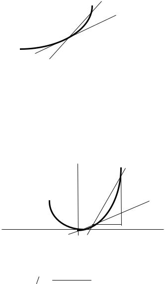
Let us first consider the problem of constructing the tangent to a curve at a given point. If we are given a curve and two points P and Q on it, it is a simple matter to draw the line or chord passing through them. As Q approaches P, the chord PQ,
|
Q |
chord |
tangent |
P |
|
Suitably produced, evidently provides a better and better approximation to the tangent at P. However, the chord PQ will differ (in general) from the tangent at P unless P and Q coincide. But when P and Q are coincident, they do not determine a unique line, since there are infinitely many straight lines passing through a given point. In the modern version of the differential calculus this problem is circumvented by obtaining the tangent to the curve at P as the line that limits the position of the chord PQ as Q approaches P—limiting in the sense that the angle between the tangent at P and the chord PQ can be made as small as we please by taking Q sufficiently close to P.
As an example, let us determine the slope of the tangent at the point P = (x0, y0) on the parabola y = x2. Let Q be the point (x0+δx, y0+ δy), where δx, δy are
|
Q |
y = x2 |
T |
|
δy |
|
P |
|
δx |
|
O |
small increments in x0 , y0 respectively. The slope of the chord PQ is given by the equation
δy δx = |
(x |
+δx)2 − x2 |
|
0 |
|
0 = 2x +δx. |
|
|
|
δx |
0 |
|
|
|
|

THE CALCULUS AND MATHEMATICAL ANALYSIS |
153 |
When Q is close to P, the increment δx is small, and by making it small enough we can bring Q as close to P as we please. Let PT be the line through P whose slope is 2x0. Then this line PT is the tangent at P, because the slope of PT is 2x0, that of PQ is 2x0 + δx, and we can take Q so close to P that the difference between these two slopes, namely δx, will be as small as we please. The slope of the tangent at (x0, y0) is, accordingly, that of PT, namely 2x0.
The process by which we passed from the slope δy/δx of the chord PQ to the slope of the tangent at P is known as the method of limits. Thus, in our example above, where δy/δx is equal to 2x0 + δx, the slope of the tangent, namely 2x0, is said to be the limit of the slope 2x0 + δx as δx tends to zero. In this definition, there is present a quantity δx which we suppose assumes smaller and smaller values tending towards zero, that is, δx is a variable tending to zero. In a figurative sense, δx may be thought of as an infinitesimal quantity.
The concept of limit, one of the most important and far-reaching in mathematics, is extended to arbitrary functions as follows. Given a function y = f(x) , we say that A is the limit of f(x) as x tends to a if the difference between f(x) and A remains as small as we please so long as x remains sufficiently near to a, while remaining distinct from a. The notation for a limit is lim, and the statement that the function y = f(x) has limit A as x tends to a is then written
lim f (x) = A |
(1) |
x→a |
|
In the nineteenth century, assertion (1) was provided with a watertight definition: the function y = f(x) is said to have limit A as x tends to a if corresponding to any ε > 0 there is δ > 0 for which1 |f(x) – A|< ε whenever 0 < |x – a| < δ. Further, we say that y = f(x) has a limit as x → a, or that the limit exists, if there is a number A for which (1) holds.
Intuitively, the gradient of a function at a point is the slope of the tangent— assuming it to be well-defined—at that point to the curve determined by the function. This is given the following precise definition in terms of the limit concept. The function y = f(x) is said to have a gradient or to be differentiable at x = x0 if the limit as δx tends to 0 of the function
f (x0 +δx) − f (x0 )
δx
exists. This limit, which is called the gradient of y = f(x) at x = x0., is often written in the less accurate but more suggestive form
lim δx→ 0 δy/δx. |
(2) |
1 If r is a real number, we write |r| for the absolute value of r, that is, |r| = r if r is positive, and |r| = –r if r is negative.
154 |
CHAPTER 9 |
If f is differentiable at each point of its domain, then its gradient is a function of the argument x, being the function which associates, with each value of x, the slope of the tangent to the curve determined by f(x). This function is called the derivative or differential coefficient of f(x) with respect to x, and is written variously as Df(x), Dy,
f′(x) or dy/dx, the latter notation being suggested by analogy with the expression in (2)
above. The process of obtaining the differential coefficient is called differentiation.
In passing we note that a function differentiable at a point is also continuous at that point. Here y= f(x) is said to be continuous at x = a if
lim f (x) = f (a).
x→a
This means simply that the curve determined by f does not have a “jump” or “gap” at x = a.
It is now straightforward to establish the usual laws for differentiation, for example:
D(axn) = naxn–1,
and, if u(x) and v(x) are both functions of x, then
D(uv) = uDv + vDu.
If we calculate the value of δy/δx defined above for various functions y = f(x), we find that in every case it consists of two terms, namely (i) the derivative, and (ii) a term of the form Ax0. Accordingly, we have, for any value of x, an equation of the form
δy/δx = f ′(x) + A x.
If we multiply this equation by x, we obtain
δy = f ′(x)δx + A(δx)2. |
(3) |
Now if δx is small, (δx)2 is considerably smaller, and it follows that f ′(x)δx is a good
approximation to δy. In recent years an approach to the calculus has been developed on the assumption of the presence of quantities δx which, while not actually being equal to zero, are nevertheless so small that their squares (δx)2 are literally equal to zero. Quantities of this sort are called square zero or nilsquare infinitesimals: for any such quantity δx equation (3) becomes
f(x + δx) – f(x) = y = f ′(x)δx.
THE CALCULUS AND MATHEMATICAL ANALYSIS |
155 |
In other words the change in the value of f(x) attendant upon a nilsquare infinitesimal change δx in x is not merely approximately, but exactly equal to f ′(x)δx. This enables
the derivative f ′(x) to be defined as that number H which satisfies the equation
f(x + δx) – f(x) = Hδx
for all nilsquare infinitesimal δx. This approach, which does not involve limits, considerably simplifies the development of the differential calculus: a further account of these ideas is given in Appendix 3.
The derivative of a function y = f(x) of x is itself a function of x and so may itself have a derivative. For example, if y = x4, then Dy = 4x3, so that D(Dy) = 12x2. The function D(Dy), in this case, 12x2, is called the second derivative of y and is written
D2y, d2y/dx2, or f′′(x). Similarly, D(12x2), that is, 24x, is called the third derivative of
y = x4 . This process may be iterated indefinitely to yield, for each natural number n, the nth derivative Dny or f (n)(y) of y = f(x).
Use of the derivative enables various physical concepts to be given precise mathematical formulations. For example, suppose that at time t (seconds) from a given instant, a body of mass m (kilos), moving in a straight line, is at distance x (metres) from a fixed point O on the line. If the velocity of the body is v (metres per second) and the acceleration a (metres per second per second), then
v = dx/dt a = dv/dt = d2x/dt2.
That is, velocity is the time derivative of distance, and acceleration is the time derivative of velocity, or the second time derivative of distance.
Newton called v the fluxion of x and a the second fluxion of x; x and v he also called the fluents (i.e., “flowing quantities”). His notation for a fluxion was a dot placed over the fluent; thus
• |
• •• |
v = x |
a = v = x |
By his second law of motion, the force F in the direction of motion is the time rate of change of the momentum mv. Therefore
F = d(mv)/dt = mdv/dt = ma.
This equation is the mathematical presentation of Newton’s second law.
An important application of the differential calculus is in determining maximum and minimum values. The method goes back in essence to Fermat. Suppose we are given a
function y = f(x); then the value of its derivative f′(x0) at x0 is the slope of the (tangent to the) curve represented by y = f(x) at x0. If f′(x0) = 0, then the curve is said to have a
stationary point at x0. It is obvious that a point at which f assumes a maximum or minimum value must be a stationary point: this fact makes the determination of these values a simple matter, as the following example illustrates.
156 |
CHAPTER 9 |
Suppose that a closed cylindrical can is to be made to contain a given volume V, and we want to determine the shape of the can so that the amount of material used in its manufacture is a minimum. We proceed as follows. Writing r for the radius of the can's base and h for its height, its total surface area is then
S = 2πrh + 2πr2.
Thus the problem is to minimize 2πrh + 2πr2, subject to the constraint V = r2h. Here we may simplify the algebra by saying that the problem is to minimize rh + r2 subject to r2h = c. If we write
f(r) = r2 + rh = r2 + c/r,
then
f′(r) = 2r – c/r2,
so that f′(r)= 0 if 2r3 = c. Thus a stationary point for f(r) is obtained when 2r3 = c, i.e.
when 2r3 = r2h, so that h = 2r. This value is a minimum because it is plain that f(r) increases indefinitely both when r tends to zero and when r increases indefinitely. We conclude that the surface area, and hence also the amount of material, is a minimum when the can’s height and base diameter coincide.
We turn now to the problem of quadrature, that is, of determining the area enclosed in, or bounded by, a curve. Thus (to follow Newton) let CPD be the graph of the function y = f(x), OA = a, AC = f(a), OM = x, MP = f(x). Let z denote the area AMPC; this area may be thought of as being generated by a line parallel to the y-axis
y |
S |
Q |
|
|
|
|
|
||
|
P |
R |
|
|
|
C |
|
D |
|
O |
A M |
N |
B |
x |
which sets out from the position AC and moves to the right. Thus z is a function of x which is zero when x = a. We wish to calculate z, and to do this we find dz/dx. (For simplicity we assume that f(x) is always positive.) When x is increased by the amount δx (= MN), the area z increases by the amount δz (= area MNQP). Draw PR, SQ parallel to MN. Then MNQP is equal to the rectangle MNRP, together with the area PRQ, which is less than the area of the rectangle PRQS; therefore
δz = MP. δx + a quantity < RQ. δx,
THE CALCULUS AND MATHEMATICAL ANALYSIS |
157 |
so that
δz/ δx = MP + a quantity < RQ.
As δx tends to zero, so does RQ, and accordingly
dz/dx = MP = f(x). |
(4) |
Note incidentally that the use of nilsquare infinitesimals makes this demonstration even simpler, for when δx is nilsquare, the area of PRQ, being proportional to (δx)2, is literally zero. Therefore z = MP. x: since this holds for arbitrary x, equation (4) again follows (see Appendix 3).
The area z under the curve y = f(x) is therefore that function of x whose derivative is f(x) (and which vanishes when x = a). We write
z = ∫ f (x)dx
reading the right-hand side of this equation as the (indefinite) integral of f(x); the operation of forming the integral is called integration. By definition the operation of differentiation is inverse to that of integration, i.e.,
d/dx[z = ∫ f (x)dx] = f(x).
The theorem that we have just demonstrated, namely, that the derivative of the function representing the area under a curve given by y = f(x) is just f(x) itself, is called the Fundamental Theorem of the Calculus: it forges the link between the two types of problem—that of tangents and that of quadrature—with which we began our discussion.
Returning to our figure on the previous page, there is a special notation for the integral that is equal to the area ABDC, namely,
b
∫ f (x)dx .
a
This is called a definite integral; it is computed by finding the indefinite integral of f(x), replacing x by b, then by a, and subtracting the second result from the first.
For example, the area under the curve y = 4x3 + 3x2 + 2x between x = 0 and x = 2 is calculated as follows. Since
d/dx[x4 + x3 + x2] = 4x3 + 3x2 + 2x,
it follows from the definition of the integral that
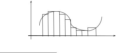
158 |
CHAPTER 9 |
∫(4x3 +3x2 +2x)dx = x4 + x3 + x2,
so the area in question is
2
∫(4x3 +3x2 +2x)dx = (4x3 + 3x2 + 2x)dx = (x4 + x3 + x2)x=2 – (x4 + x3 + x2)x=0
0
= 24 + 23 + 22 – 0 = 28.
The interpretation of the area z under a curve will depend on the nature of the quantities represented by x and y. Here are some examples.
(i)If OM or x represents time and MP velocity, then the area z represents the gain in distance during the time represented by AM.
(ii)If OM represents time and MP acceleration, then z represents the velocity gained in the time represented by AM.
(iii)If OM represents the distance a force moves its point of application and MP the force, then z represents the work done by the force in moving its point of application through the distance represented by AM.
(iv)If OM represents time and MP the temperature in a room, then z represents the total energy expended in heating the room during the time represented2 by AM.
There is an alternative way of arriving at the definite integral, namely as the limit of a sum, a method which, in essence at least, goes back to the ancient Greek method of exhaustion but which in its modern form is due to Riemann. Thus, consider once again the curve defined by the function y = f(x) between x = a and x = b. We will see first how the area under the curve, which we shall now denote by A, can be approximated by a sum of rectangles. We divide the interval from a to b into N small subintervals (xm, xm+1), of equal width (b – a)/N, with x0 = a and xn = b, and define δx = xm – xm–1` = (b – a)/N. We choose δx as the common length of the bases of
y
O |
a |
xm |
b |
x |
2Thus the energy expended in heating a room over a stretch of time depends only on the average temperature during that time: when one is out it is cheaper to turn the thermostat down and allow the room to cool than to maintain it at a constant temperature, even though the process of reheating it on one’s return may require a
disconcertingly steady expenditure of heat energy.

THE CALCULUS AND MATHEMATICAL ANALYSIS |
159 |
our “approximating rectangles”. As their heights we choose the value of y = f(x) at the right-hand endpoint of the subinterval. Thus the sum of the areas of these rectangles will be
SN = f(x1)δx + f(x2)δx + ... + f(xN)δx,
which we abbreviate as 3
N
SN = ∑ f (xj )δx .
j =1
Now we form a sequence of such approximations in which N increases indefinitely, so that the number of terms in each sum increases while, owing to the presence of the factor δx = (b – a)/N, each single term f(xj)δx tends to zero. By taking N sufficiently large, we can make SN differ from the area A by an amount as small as we please. This we express briefly by saying that A is the limit of the SN as N tends to infinity. We may
b |
N |
)δx |
then define the definite integral ∫ f (x)dx = A as the limit of the sums SN = |
∑ f (xj |
|
a |
j =1 |
|
as N tends to infinity.
Leibniz symbolized this passage to the limit from the approximating sum SN to A by replacing the summation sign ∑ —which in his time was written “S”—by the symbol
∫ (a stylized “S”), and the difference symbol δ by the symbol d. This notation is
standard today.
The natural logarithm log(x) is an important example of a function defined by means of integration. It is defined for positive x by
x dt
log(x) = ∫
1 t
The number e—like π, one of the fundamental constants of mathematics—is defined to be that number whose logarithm is 1, that is,
e dt
1 = ∫
1 t
e has the value 2.7182818…. The function ex, also written exp(x), is called the
exponential function; it can be shown that ex is the function inverse to log(x), that is, elog(x) = log(ex) = x. The exponential function has the key property of being equal to its
own derivative: D(ex) = ex.
3Here the symbol ∑N signifies the sum of all the expressions obtained by allowing j to assume successively
j =1
the values 1, 2, 3,.., N.

160 |
CHAPTER 9 |
The definition of the integral as the limit of a sum of plane areas can be extended to three (and higher) dimensions so as to enable the differential calculus to be employed in determining areas of curved surfaces and volumes of solids. This definition also provides the basis for the general theories of integration which have been developed in the present century.
MATHEMATICAL ANALYSIS
Within both the differential and integral calculus the limit concept plays a central role: the derivative of a function is the limit of a quotient, and the definite integral is the limit of a sum. A characteristic feature of the limit concept is that it involves the idea of an infinite process: in forming a limit as x tends to zero, say, we imagine x becoming smaller and smaller endlessly without ever actually vanishing. The use of infinite processes is the hallmark of the extensive area of mathematics known as mathematical analysis, or analysis for short. Analysis may be considered, along with geometry and algebra (here taken to include number theory), as one of the three main divisions of mathematics. Analysis is, perhaps, the largest of these divisions, and includes many topics besides the calculus; only a few of these will be touched on here. We defer until Chapter 11 our discussion of set theory, the branch of mathematics concerned with the infinite in its purest form, and which may be considered to have emerged from analysis.
Infinite Series
Let a0, a1, a2, … be a sequence of real numbers. We say that the sequence—which we shall denote by <an>—converges to limit a as n tends to infinity—written an → a as4
n →∞—if the differences between an and a become arbitrarily small as n becomes arbitrarily large. To be precise, <an> converges to limit a if, corresponding to any ε > 0 there is an integer N such that |an – a| < ε for all n ≥ N. In the opposite event, the
sequence is said to diverge.
Given a sequence <an>, the sequence <Sn> defined by
n
Sn = ∑ aj = a1 + a2 + … + an
j =1
is called the sequence of partial sums of the infinite series
∞
∑ an ,
n=1
4 The sign “∞” to denote an infinite number was introduced by Wallis in his work De Sectionibus Conicis of 1655. It has been conjectured that Wallis, who was a classical scholar, adopted this sign from the late Roman symbol “∞” (possibly a form of “M”) for 1000.
THE CALCULUS AND MATHEMATICAL ANALYSIS |
161 |
sometimes written simply
∑an .
If Sn → s as n → ∞, the series is said to converge to the sum s, and we write
∞
s = ∑ an = a1 + a2 + … + an + … .
n=1
In the opposite event the series is said to diverge.
The most familiar type of convergent series is the geometric series
∞
∑ xn
n=1
with fixed x satisfying |x| < 1. In this case the partial sums satisfy
Sn |
= ∑ x j =1+ x +... + xn = 1− x |
n+1 |
||
. |
||||
|
n |
|
|
|
|
j =1 |
1− x |
|
|
If |x| < 1, then xn+1 → 0 as n → ∞, so that
Sn → 1/(1 – x) as n → ∞.
∞
Accordingly ∑ xn converges with sum 1/(1 – x) provided |x| < 1.
n=1
The ancient Greeks were conversant with the idea that an infinite series could converge, even if they lacked a precise definition of the concept. In particular they had grasped the fact that
12 + 14 + 18 +...+ 12n +... =1.
In Chapter 6 of his Physics Aristotle observes, in effect, that such a series should have a sum.
Infinite series make an occasional appearance in medieval mathematics. Nicolas Oresme (c. 1323–1382), for example, observed that the so-called harmonic series
12 + 13 + 14 +...1n +...
is divergent. For it can be replaced by the series of lesser terms
(14 + 14) +(18 + 18 + 18 + 18) +...,
162 |
CHAPTER 9 |
which yields as many terms of magnitude ½ as one pleases.
In 1593 Viète derived a formula for the sum of an infinite geometric series, and in 1647 Gregory of St. Vincent (1584–1687), in his Opus Geometricum, is the first to state explicitly that a convergent infinite series represents a magnitude, which he calls the limit of the series.
The principal use of infinite series has been to represent functions, and thereby to provide a means for calculating their values. In the mid-seventeenth century, for instance, Newton obtained a series for the natural logarithm
log(1 + x) = x − 12 x2 + 13 x3 −...,
which converges for |x| ≤ 1. This is a typical example of what is known as a power series. Newton also obtained the power series
x |
= 1+ x + |
x2 |
x3 |
|
||
e |
|
+ |
|
+... , |
(1) |
|
2! |
3! |
|||||
so that in particular
e = 1+1+ 2!1 + 3!1 +... ,
as well as power series for the trigonometric functions5
sin x = x − |
x3 |
x5 |
(2) |
|||||
|
+ |
|
|
−... |
||||
3! |
5! |
|||||||
|
|
|
|
|
|
|||
cos x = 1− |
|
x2 |
x4 |
|
||||
|
|
+ |
|
|
−... . |
(3) |
||
|
2! |
4! |
|
|||||
|
|
|
|
|
|
|||
An important general method, still very much in use today, for representing a function as a power series was developed by Brook Taylor (1685–1731) in his
Methodus Incrementum Directa et Inversa of 1715. Building on the work of Newton and James Gregory, Taylor obtains for the function y = f(x) the equation
f(x + h) = f (x) + hf '(x) + h2 f ''(x) + h3 f '''(x) +...
2! 3!
Putting x = 0 yields the equation
5 Here sin x and cos x are given as functions of a variable angle x measured in radians, where a radian is the angle subtended at the centre of a circle by an arc equal to the radius. Thus π radians = 180°.
THE CALCULUS AND MATHEMATICAL ANALYSIS |
163 |
|||||
f(h) = |
f (0) +hf '(0) + |
h2 |
f ''(0) + |
h3 |
f '''(0) +... |
|
2! |
3! |
|
||||
|
|
|
|
|
||
This is known as Maclaurin’s theorem, after Colin Maclaurin (1698–1746). In obtaining their series neither Taylor nor Maclaurin employ rigorous argument, nor do they consider the question of convergence. Maclaurin derives his series by means of the method of undetermined coefficients. He begins by assuming that f(x) can be expanded as a series
f(x) = A + Bx + Cx2 + Dx3 + … .
Then by successive term-by-term differentiation he obtains
f′(x) = B + 2Cx + 3Dx2 + … . f′′(x) = 2C + 6Dx + … .
Putting x = 0 in each equation then determines A, B, C, D, ….
Euler was the master of infinite series. These he would manipulate with great flair, only rarely paying attention to the question of convergence. In his Introductio in Analysin Infinitorum of 1748 are to be found many examples of his skill in this regard. One of his most famous results obtained by the formal manipulation of infinite series relates the exponential and logarithmic functions through complex numbers and is known as the Euler identity, namely,
eix = cos x + i sin x. |
(4) |
This memorable equation may be derived by noting that, if we substitute ix for x in the series expansion (1) for ex and use the series expansions (2) and (3) for sin x and cos x, we get
ix |
= 1+ix − |
|
x2 |
|
ix3 |
x4 |
ix5 |
|
|
|
|||||||
e |
|
|
− |
|
|
+ |
|
+ |
|
+... |
|
||||||
|
2! |
|
3! |
4! |
5! |
|
|||||||||||
|
= |
(1− |
x2 |
+ |
x4 |
|
−...) +i(x |
− |
x3 |
+ |
x5 |
−...) |
|||||
|
2! |
4! |
3! |
5! |
|||||||||||||
|
|
|
|
|
|
|
|
|
|
|
|||||||
|
= |
cos x + i sin x. |
|
|
|
|
|
|
|
|
|||||||
If we substitute π for x in (4), and note that cos π = –1, sin π = 0, we obtain one of the most remarkable equations in the whole of mathematics, namely,
eiπ + 1 = 0.
Of course, equations such as this only become meaningful when quantities such as eiπ are properly defined: this was not carried out until the nineteenth century.
164 |
CHAPTER 9 |
Using his freewheeling methods, Euler was able to achieve results which baffled his contemporaries. One of his most remarkable feats was the summing of the series
112 + 212 + 312 +... . To effect this, Euler began with the equation (2) for sin x; the
equation sin x = 0 can then be thought of—after dividing through by x—as the infinite polynomial equation
0 = 1− x2 + x4 −...
3! 5!
or, replacing x2 by y,
0 = 1− y + y2 −...
3! 5!
From the theory of algebraic equations it is known (and not difficult to show) that if the constant term in a polynomial equation is 1, then the sum of the reciprocals of the roots
is the negative of the coefficient of the linear term, which in this case is 3!1 . Moreover,
the roots of the equation sin x = 0 are known to be π, 2π, 3π,…; accordingly, the roots of the equation in y are π2, (2π)2, (3π)2, … . Therefore
61 = π12 + (21π)2 + (3π1)2 +...
or
π2 |
= |
1 |
+ |
1 |
+ |
1 |
+... |
(5) |
||
6 |
|
2 |
2 |
2 |
2 |
|||||
|
1 |
|
|
|
3 |
|
|
|||
Using the cosine series (4) in place of the sine series, Euler similarly obtained the result
π2 |
= |
1 |
+ |
1 |
+ |
1 |
+... |
(6) |
||
8 |
|
2 |
2 |
5 |
2 |
|||||
|
1 |
|
3 |
|
|
|
|
|||
Subtracting equation (5) from twice equation (6) gives
π2 = 1 − 1 + 1 − 1 +...
12 12 22 32 42
These arguments, while hardly rigorous, are nothing less than spectacular. In the nineteenth century, the great majority of Euler’s results were derived by rigorous, but less entertaining methods.
THE CALCULUS AND MATHEMATICAL ANALYSIS |
165 |
An important class of infinite series are the so-called trigonometric series, which had first arisen in connection with the analysis of planetary orbits. By a trigonometric series is meant any series of the form
∞
12 a0 + ∑ (an cos nx +bn sin nx) .
n=1
Each of the sine and cosine functions in this series has a wave-like or “sinusoidal” graph of the form
Thus the function represented by such a series is a “superposition” of such waves. Trigonometric series were investigated in the eighteenth century by Euler,
Jean–le–Rond d’Alembert (1717–1783), Clairaut, and Lagrange, but it was Joseph Fourier (1768–1831)—in his papers of 1807, 1811, and above all in his celebrated work Théorie Analytique de la Chaleur of 1822—who first advanced the claim that an arbitrary function y = f(x) can be represented as a trigonometric series, thus introducing the branch of mathematics that has become known as harmonic analysis. Fourier obtains the expressions (in which he was anticipated by Euler)
a |
= 1 |
2π |
b |
|
= 1 |
2π |
∫ f (x)cos nx dx |
n |
∫ f (x)sin nx dx |
||||
n |
π |
0 |
|
π |
0 |
|
|
|
|
|
|
for the coefficients of the trigonometric series expansion of f(x). Fourier’s work was so influential that the trigonometric series representing a function is called its Fourier expansion and the coefficients of this series its Fourier coefficients.
Fourier did not supply a rigorous proof that the trigonometric series associated with a function converges to the value of the function, and later work showed that for certain functions this was not in fact the case. It was Dirichlet who, in 1828, gave the first rigorous proof of convergence of the Fourier expansion of a function subject to certain restrictions. He showed that, if y = f(x) is continuous at each point of its domain,
π
periodic of period 2π, that is, f(x + 2π) = f(x), and ∫ f (x)dx is finite, then the Fourier
−π
expansion of f always converges to f(x).
The mathematicians of the eighteenth century had been somewhat cavalier in their use of infinite series, and by the century’s end certain dubious or downright absurd results obtained by their means provoked enquiries as to the validity of operating with them. In the forefront of these investigations was Cauchy, who in his Cours d’Analyse of 1821 gave the rigorous definition of convergence of an infinite series employed
166 |
CHAPTER 9 |
today, and who also formulated the purely internal criterion for convergence which has come to bear his name (although it was known earlier to Bolzano). This states that a necessary and sufficient condition that an infinite series ∑an converge is that, for any
given value of p, the difference between the partial sums Sn and Sn+p tends to zero as n tends to infinity.
While the injection of rigor into the theory of infinite series administered in the nineteenth century may have tamed the subject, it has remained colourful. The resulting precision also made possible the discovery of new and striking facts about infinite series. Riemann’s theorem is an example. This stems from the observation that certain series containing positive and negative terms exist with the property that, while they converge, the series obtained by making all their terms positive do not. For instance,
1− 12 + 13 −14 +...
converges to log 2, but, as we have seen, the corresponding series of positive terms
1+ 12 + 13 + 14 +...
diverges to infinity. A series of this type is called conditionally convergent. Riemann’s theorem asserts that, given any conditionally convergent series, its terms can be rearranged so that the resulting series converges to any value whatever. Thus, for example, it can be shown that
1 + 13 −12 + 15 + 17 −14 +... = 3 2 log(2)
and
1 − 12 −14 + 13 − 16 + 18 +... = 12 log(2) .
Differential Equations
In the seventeenth and eighteenth centuries mathematicians applied the calculus to a broader and broader range of physical problems. The mathematical formulation of many of these problems involved what came to be known as differential equations, that is, equations involving derivatives of a function or functions, from which the functions themselves are to be determined.
A general problem of this sort is the following. Consider a material particle of mass m moving along a line, and let x denote its distance at time t from some given fixed point on the line. Let us assume that the motion is caused by some force F, the value of which depends on x, on the velocity dx/dt, and on the time t; to indicate this dependence we write F = F(x, dx/dt, t). According to Newton’s second law of motion,

THE CALCULUS AND MATHEMATICAL ANALYSIS |
167 |
the action of the force F on the particle produces an acceleration a = d2x/dt2 with |
F = |
ma, and so we obtain the differential equation |
|
Md2x/dt2 = F(x, dx/dt, t). |
(1) |
More specifically, let us suppose that the particle is moving in a resisting medium, for example in a liquid or a gas, under the influence of the elastic force of two springs, acting in accordance with Hooke’s law (after Robert Hooke, 1635–1703), which states that the elastic force of a spring acts towards the equilibrium position and is proportional to the deviation therefrom. Assuming that the equilibrium position is at x = 0, the elastic force is then proportional to –bx, where b is some positive constant. We also suppose that the resistance of the medium is proportional to the speed of the motion, that is, equal to –adx/dt, where a is some positive constant. In that case the force F acting on the particle is –bx – adx/dt and so equation (1) assumes the form
m d2x/dt2 + a dx/dt + bx = 0.
This is the differential equation of motion of the particle. Its solution x = x(t) gives the position x of the particle as a function of the time t.
Differential equations also arise in the determination of the form of curves. For example, in 1690 Jacques Bernoulli posed the problem of finding the curve assumed by a flexible inextensible cord hanging freely from two fixed points, the curve Leibniz named the catenary. This problem had been considered as far back as the fifteenth century by Leonardo da Vinci; Galileo mistakenly thought that the curve was a parabola. Huygens showed that this was not correct and that the curve would assume a parabolic form only when the combined weight of the cord and any objects suspended from it is uniform per horizontal run, as in a suspension bridge. In 1691 Leibniz, Huygens and Jean Bernoulli published independent solutions to the problem, the latter employing the methods of the calculus. Writing y = f(x) for the equation of the curve, Bernoulli obtains the differential equation
1 + (dy/dx)2 = a2y,
and gives the correct solution
y = ½a(ex/a – e–x/a).
Perhaps the most celebrated solution to a set of differential equations is Newton’s derivation of Kepler’s laws of planetary motion. Formulated in 1609 and 1619 by Johannes Kepler (1571–1630), these laws are the following three assertions:
1. The planets move about the sun in elliptical orbits with the sun at one focus6.
6 An ellipse may be defined as the locus of all points the sum of whose distances from two given points is constant: these two points are the foci of the ellipse.
168 |
CHAPTER 9 |
2.The radius vector joining a planet to the sun sweeps over equal areas in equal intervals of time.
3.The square of the time of one complete revolution of a planet about its orbit is proportional to the cube of the orbit’s semimajor axis.
In his Philosophiae Naturalis Principia Mathematica—universally known as the
Principia—of 1687, Newton formulates his laws of motion and the inverse square law of gravitational attraction between two bodies, and from them deduces Kepler’s laws, at the same time creating the science of celestial mechanics. Although Newton casts his work in the form of classical Greek geometry, it is almost certain that he obtained his results in the first instance by the use of the calculus, which means, in essence, that he solved the differential equations of motion of a body moving under a central force.
Partial differential equations are also frequently encountered in physics. These are equations involving partial derivatives. If f(x, y, z, …) is a function of the variables x, y,
z, …, the partial derivative ∂∂fx of f with respect to one of these variables, x, say, is obtained by fixing the values of the remaining variables y, z, …, and then
differentiating |
the resulting function of x. |
Similarly one obtains higher partial |
||||
derivatives |
∂2 |
f |
and mixed partial derivatives |
∂2 f |
. It is a fundamental property of |
|
∂x2 |
∂x∂y |
|||||
|
|
|
||||
partial differentiation that the order in which the differentiations are made is irrelevant:
thus, for example, ∂2 f = ∂2 f .
∂x∂y ∂y∂x
One of the first, and undoubtedly most important, partial differential equations—the wave equation—made its appearance in the eighteenth century in connection with the analysis of a vibrating string, a violin string, for example. In 1746 d’Alembert gave the correct form of the equation governing a flexible continuous vibrating string:
T |
∂2u |
= ρ |
∂2u |
(2) |
|
∂x2 |
∂t2 |
||||
|
|
|
where u = u(x, t) is the displacement of the string from its equilibrium position at time t and position x along it, T is the tension in the string and ρ is its density. D’Alembert shows that (2) has a solution of the form
u(x, t) = ϕ(ct + x) + ψ(ct – x),
where c = T ρ and ϕ, ψ are arbitrary twice differentiable functions. This solution
may be considered as the superposition of two “standing waves”, each moving in opposite directions along the string.
In 1748 Euler gave a solution to the wave equation in the form of a trigonometric series

THE CALCULUS AND MATHEMATICAL ANALYSIS |
169 |
u(x, t) = ∑ An sin nπx A cos nπct A.
This solution presents the characteristic vibrations of the string in terms of a superposition of infinitely many elementary wave motions of sinusoidal form.
Later the wave equation was extended to three spatial dimensions, taking the form
∂2u |
+ |
∂2u |
+ |
∂2u |
= c |
2 |
∂2u |
. |
∂x2 |
∂y2 |
∂z2 |
|
∂t2 |
||||
|
|
|
|
|
This equation, one of the most important in mathematical physics, governs the vibrations of solid bodies and the propagation of waves such as sound and light.
Another important partial differential equation in mathematical physics is the potential equation, also known as Laplace’s equation, which takes the form
∂2V + ∂2V + ∂2V = 0. ∂x2 ∂y2 ∂z2
This equation, which was given in 1789 by Pierre Simon de Laplace (1749–1827), governs the gravitational potential V(x, y, z) outside a gravitating body. The potential function V(x, y, z) is characterized by the property that its partial derivatives with respect to the three spatial coordinates x, y and z are the three components of the gravitational force exerted by the body at the point (x, y, z).
Other important partial differential equations arise in connection with fluid flow. In a paper of 1755 entitled General Principles of the Motion of Fluids, Euler derives his famous equations of flow for perfect nonviscous fluids. If we write u, v, w for the components of the velocity of the fluid at time t in the x, y and z directions, p for the pressure and ρ for the density of the fluid, the first of Euler’s equations for compressible flow takes the form
∂p |
|
|
∂u |
+v |
∂u |
+ w |
∂u |
+ |
∂u |
∂x |
= −ρ u |
∂x |
∂y |
∂z |
|
||||
|
|
|
|
|
∂t |
||||
with analogous expressions for |
∂p and |
∂p |
. Euler also obtains a general form of the |
||||||
|
|
∂y |
|
∂z |
|
|
|
|
|
so-called equation of continuity which had been derived previously by d’Alembert for incompressible flow, and which expresses the fact that matter is neither created nor destroyed in fluid motion. Euler’s version of the equation is:
∂∂pt + ∂(∂ρxu) + ∂(∂ρyv) + ∂(∂ρzw) = 0.
For incompressible flow ρ is constant and we obtain d’Alembert’s form of the equation
170 |
CHAPTER 9 |
∂∂ux + ∂∂yv + ∂∂wz = 0.
If we follow Euler by introducing a function S, called the velocity potential, whose partial derivatives with respect to x, y, and z are u, v and w, respectively, we see that S satisfies Laplace’s equation. This equation is also characteristic of fluid flow.
Finally, we must mention the heat equation which was obtained by Fourier in his Théorie Analytique de la Chaleur. By physical arguments, Fourier showed that the temperature T at a point (x, y, z) at time t in a homogeneous and isotropic body satisfies the equation
∂2T |
+ |
∂2T |
+ |
∂2T |
= k |
2 |
∂T |
, |
∂x2 |
∂y2 |
∂z2 |
|
∂t |
||||
|
|
|
|
|
where k is a constant whose value depends on the material of the body. When T is independent of the time, ∂∂Tt = 0 and the equation reduces to Laplace’s equation. In one
dimension Fourier gave a solution to the equation in the form of a trigonometric series with exponential coefficients
T = ∑bnexp(−n2 π2 k2 A2 )t sin nπx A.
The presence of the exponential terms here reflects the fact that, as a body cools, its temperature falls off as e–kt with the time t.
Complex Analysis
One of the most significant and original mathematical creations of the nineteenth century was the theory of functions of a complex variable, or complex analysis for short. Now, strictly speaking, a function of a complex variable is just a function
f: ^ → ^, so that, for each z = x + iy, f(z) is a complex number whose real and
imaginary parts are uniquely determined by x and y. In other words, there are functions u(x, y) and v(x, y) of two real variables x and y such that f(x + iy) = u(x, y) + iv(x, y). Thus, according to this definition, a complex function is essentially nothing more than a pair of real functions.
Both Cauchy and Riemann independently saw that this definition, while perfectly legitimate, was too broad to be of much practical value. They proposed instead that attention be confined to complex functions which are differentiable in the same sense
as real functions. Thus a function f: D → ^, where D is a region in the complex plane is said to be differentiable at a point z0 of D if
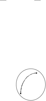
THE CALCULUS AND MATHEMATICAL ANALYSIS |
171 |
||
|
f (z) − f (z0 ) |
|
(1) |
|
z − z0 |
||
|
|
||
tends to a unique limit as z → z0. A function which is differentiable in this sense at every point of a region D is said to be analytic (also: regular or holomorphic) on D.
Since analyticity requires that (1) has a unique limit when z – z0 tends to zero not merely through purely real or purely imaginary values, but along any path whatsoever, it is evidently a very strong condition. Cauchy and Riemann independently discovered that the real and imaginary parts u(x, y) and v(x, y) of an analytic function satisfy what are now known as the Cauchy–Riemann equations, viz.,
∂u |
= |
∂v |
∂u |
= − |
∂v . |
∂x |
|
∂y |
∂y |
|
∂x |
And conversely, if u and v are continuous and have continuous partial derivatives satisfying the Cauchy-Riemann equations throughout a region, then f = u + iv is analytic in that region.
From the Cauchy-Riemann equations we deduce, by partial differentiation,
∂2v = ∂2u = − ∂2u ∂x∂y ∂x2 ∂y2
∂2u = − ∂2v = − ∂2v . ∂x∂y ∂x2 ∂y2
Accordingly both u and v satisfy the two-dimensional version of Laplace’s equation, that is
∂2V + ∂2V = 0. ∂x2 ∂y2
It follows that, by separating any analytic function into its real and imaginary parts, two solutions of Laplace’s equation are immediately obtained. It is this fact that makes complex analysis so useful in the solution of problems in mathematical physics, especially in the theory of fluid flow.
Cauchy proved what is perhaps the single most important result of complex analysis, now known as the Cauchy integral theorem. Given a curve C in a region of the complex plane, the integral of an analytic function f along C may be defined in a manner analogous to that of the definite integral of a real function. Namely, if a, b are
b
y tn–1
yC
y
y t2 yt1
172 |
CHAPTER 9 |
a
the endpoints of |
the curve, |
we subdivide it into n |
segments by means of the |
||||
successive points a = t0, t1, t2, …, tn = b and form the sum |
|||||||
|
|
S |
|
n |
(t* )(t −t |
), |
|
|
|
n |
= ∑ f |
|
|||
|
|
|
i=1 |
i i i−1 |
|
|
|
|
|
|
|
|
|
|
|
where t* denotes |
any point |
on |
C lying |
between |
t |
and t If we now make the |
|
i |
|
|
|
|
|
i–1 |
i. |
subdivision finer and finer by allowing the number of points to increase without limit in such a way that the greatest of the distances |ti – ti–1| tends to zero, then Sn tends to a
limit which is independent of the choice of the points ti and ti* . This limit is the integral
of f(z) along C and is written
∫C f (z)dz.
Now the Cauchy integral theorem asserts that, if f(z) is analytic in a simply connected region D of the complex plane, and C, C′are any two simple curves in D with the same end points, then
∫C f (z)dz = ∫C ' f (z)dz.
That is, the integral is independent of the path. In particular, if C is a closed curve, then
∫C f (z)dz = 0.
Cauchy’s theorem has many consequences, one of the most important of which we mention in conclusion. This is that every analytic function can be expanded as a power series. Precisely, if f(z) is analytic on and inside a simple closed curve C, then, for any given point a inside C, there are complex numbers b1, b2, … for which
f(z) = f(a) + b1(z – a) + b2(z – a)2 + …
whenever z is inside C. Notice that, since the coefficients b1, b2, … depend only on a, a function analytic in a region can be represented as a single power series, not just locally, but throughout the entire region. This shows once again what a powerful condition analyticity is.