CHAPTER 6

THE EVOLUTION OF ALGEBRA, III

Algebraic Numbers and Ideals

ONE OF THE MOST SIGNIFICANT PHASES in the development of algebra was the emergence in the nineteenth century of the theory of algebraic numbers. This theory grew from attempts to prove Fermat’s “Last Theorem” that xn + yn ≠ zn for positive integers x, y, z and n > 2 (see Chapter 3). The problem was taken up afresh in the eighteen forties by the German mathematician Ernst Eduard Kummer (1810–1893). He considered the polynomial xp + yp with p prime, and factored it into

(x + y)(x + αy)…(x +αp–1y),

where α is a complex pth root of unity (see Chapter 3), i.e., a complex solution to the equation

xp – 1 = 0.

Since

xp – 1 = (x – 1)(xp–1 + xp–2 + … + x + 1),

and α ≠ 1, α must satisfy the equation

Extending an idea of Gauss, Kummer termed a complex integer any number obtained by attaching arbitrary integers to the terms of the expression on the left side of (1), that is, any complex number of the form

ap–1αp–1 + ap–2αp–2 + … + a1α + a0,

where each ai is an ordinary integer. The complex integers then form a ring, that is, the sum and product of any of them is a number of the same form. This is clearly the case for sums, and the truth of the claim for products follows immediately from the observation that the set of numbers {1, α, … , αp–1} = P is closed under multiplication, that is, the product of any pair of members of P is again a member of P. For suppose

89

= αm+n is in P, while if m + n ≥ p, then, since αp = 1, αm.αn = αm+n = αp.αm+n–p = αm+n

and the latter is a member of P.

In this connection it is also easily shown that the set P consists of all the pth roots of unity. For clearly each member x of P satisfies xp – 1 = 0. Since there are exactly p solutions to this equation, it suffices to show that all the elements of P are distinct. To this end, suppose if possible that αm = αn with 0 ≤ m < n ≤ p – 1. Then αn–m = 1 and

0 < n – m ≤ p – 1. Now let q be the least integer such that αq = 1 and 0 < q ≤ p – 1. Then since p is prime, p may be written as sq + r with 0 < r < q, so that 1 = αp = αsq+r = αsq .αr = 1. αr = αr. This contradicts the definition of q, and shows that our original assumption that two members of P were identical was incorrect.

Kummer extended to complex integers concepts familiar for the ordinary integers such as primeness, divisibility, and the like, but then mistakenly supposed that the fundamental theorem of arithmetic holds in the ring of complex integers just as it does in the ring of ordinary integers, in other words, that every complex integer factorizes uniquely into primes. It was pointed out by P.G. Lejeune Dirichlet (1805–1859) that this is not always the case for rings of numbers.

We define a unit of a ring to be an element u for which there is an element v such that uv = 1; thus a unit is an invertible element of a ring. A factorization a = a1a2…an of an element a of a ring is called a proper factorization if none of the ai is a unit or zero. An element of a ring is then said to be prime if it has no proper factorization.

Now consider the set of numbers of the form

a + b√–5,

where a, b are integers. It is easily verified that this set is closed under addition and multiplication and so constitutes a ring, which we shall denote by ][√–5] to indicate

that it is the ring obtained by adjoining √–5 to the ring ] of integers. In ][√–5] the number 9 can be factorized in two different ways:

We claim that these are both prime factorizations in ][√–5] . To establish this, we need

Now if a + b√–5 is a unit, then there exists an element c + d√–5 such that

(a + b√–5)(c + d√–5) = 1.

a0 + a1x + …+ anxn = 0,

where the ai are integers. If an = 1, the roots are called algebraic integers. For example, (–6 + √–31)/2 is an algebraic integer because it is a root of the equation x2 + 3x + 10 = 0. It can be shown that the set of all algebraic numbers forms a field, that is, the sum, product, and difference of algebraic numbers, as well as the quotient of an algebraic number by a nonzero algebraic number, are all algebraic numbers. If u1,…, un are algebraic numbers, then the set of algebraic numbers obtained by combining u1,…, un with themselves and with the rational numbers under the four arithmetic operations is

clearly also a field: this field will be denoted by _(u1,…, un) to indicate that it has been obtained by adjoining the algebraic numbers u1,…, un to the field _ of rationals. A field of the form _(u1,…, un) is called an algebraic number field.

The set of algebraic integers in any algebraic number field _(u1,…, un) includes the ring ] of integers and is closed under all the arithmetical operations with the exception of division and therefore constitutes a ring. We denote this ring, which we call a ring of algebraic integers, by ](u1,…, un). The ring ][√–5] of algebraic integers in the field _[√–5] can be shown to coincide with the ring ][√–5] of numbers of the form

a + b√–5 discussed above: we have seen that the fundamental theorem of arithmetic fails in this ring, and so does not generally hold in rings of algebraic integers2.

Dedekind’s method of restoring unique prime factorization in rings of algebraic integers was to replace Kummer’s ideal numbers by certain sets of algebraic integers which, in recognition of Kummer, he called ideals, and to show that unique factorization, suitably formulated, held for these.

To understand Dedekind’s idea, let us turn our attention to the simplest ring of algebraic integers, the ring ] of ordinary integers. In place of any given integer m,

Dedekind considers the set (m) of all multiples of m. This set has the two characteristic properties that Dedekind requires of his ideals, namely, if a and b are two members of it, and q is any integer whatsoever, then a + b and qa are both members of it. Moreover, two sets of the form (m) can be multiplied: for if we define the product (m)(n) to be the set consisting of all multiples xy with x in (m) and y in (n), then clearly

(m)(n) = (mn).

In general, if we are given any ring R, an ideal in R is a subset I of R which is closed under addition and under multiplication by arbitrary members of R, that is, whenever x and y are in I and r is in R, x + y and rx are both members of I. Any list

2 Nevertheless there do exist rings of the form ][√–n] in which the fundamental theorem of arithmetic holds,

namely, when n = 1, 2, 3, 7, 11, 19, 43, 67, 163. Numerical evidence had strongly suggested that these were the only possible values of n, and in 1934 H. A. Heilbronn (1908–1975) and E. H. Linfoot (1905–1982) showed that there could be at most one more such value. Finally, in 1969 H. M. Stark proved that this additional value does not exist.

{a1, … , an} of elements of R generates an ideal, denoted by (a1, … , an), consisting of all elements of R of the form

r1a1 + … + rnan ,

where the ri are any elements of R. An ideal I is called principal if it is generated by a single element a, that is, if I = (a) : thus, as before, (a) consists of all the multiples of a. The zero ideal (0) consists of just 0 alone and the unit ideal (1) is, plainly, identical with R itself.

If (a) and (b) are two principal ideals, then it is readily established that (a) is included in (b) exactly when b is a divisor of a, that is, when a = rb for some r. Extending this to ideals, we say that an ideal J is a divisor of an ideal I when I is included in J. For principal ideals (a) and (b), the ideal (a, b) is easily seen to be their greatest common divisor, in the sense that (a, b) is a divisor of both (a) and (b) and any divisor of (a) and (b) is at the same time a divisor of (a, b).

Ideals may be multiplied: if I and J are ideals we define the product IJ to be the ideal consisting of all elements of the form x1 y1 +...+ xn yn , where x1 ,..., xn , y1 ,..., yn are

elements of I and J respectively. Clearly IJ is included in both I and J. An ideal I is said to be a factor of an ideal K if there is an ideal J for which IJ= K. If I is a factor of K, then I includes K (but not conversely).

An ideal P is said to be prime if—by analogy with integers—whenever P is a divisor of a product IJ of ideals I and J, then P is a divisor of I or of J. It is not difficult to show that this is equivalent to the requirement that whenever a product xy is in P, then at least one of x, y is in P.

The fundamental result of Dedekind’s ideal theory is that, in any ring of algebraic integers, every ideal can be represented uniquely, except for order, as a product of prime ideals. In particular, every integer u of the ring determines a principal ideal (u) which has such a unique factorization.

Let us illustrate this in the case of the ring ][√–5] considered above. In this ring the number 21 has the different prime factorizations

Now form the greatest common divisor of the principal ideals (3) and (1 + 2√–5): this is the ideal P1 = (3, 1 + 2√–5). Consider also the ideals

P2 = (3, 1 – 2√–5), Q1 = (7, 1 + 2√–5), Q2 = (7, 1 – 2√–5).

Each pair of these ideals may be multiplied simply by multiplying their generating elements, for instance P1 P2 = (9, 3 – 6√–5, 3 + 6√–5, 21). The ideal P1 P2 contains both the numbers 9 and 21, whose g.c.d. is 3. Hence by equation (2) on p. 57, Chapter 4, integers k and A can be found to satisfy 3 = 9k + 21 A, and it follows that 3 must be a member of P1 P2. But all four generators of P1 P2 are multiples of 3, so P1 P2 is

simply the principal ideal (3) consisting of all multiples of 3 in ][√–5] . Similar computations establish that

for instance, P1. First, we observe that the only (ordinary) integers in P1 are the multiples of 3. For if a nonmultiple of 3, m say, were in P1, then, as argued above, the g.c.d. of 3 and m, namely 1, would also be in P1. In that case there would be

elements a + b√–5, c + d√–5 of ][√–5] for which

1= 3(a + b√–5) + (1 + 2√–5)(c + d√–5).

Multiplying out the right side of this equation and equating coefficients of the terms involving, or failing to involve, respectively, √–5 gives

1 = 3a + c – 10d

0 = 3b + d + 2a.

Multiplying the first of these by 2 and subtracting the second gives 6a – 3b – 21d = 2,

an impossible relation since the left side is an integer divisible by 3. Therefore the only integers in P1 are the multiples of 3.

We also observe that, since P1 is a factor of P1 Q2 = (4 – √–5) = (√–5 – 4), the number √–5 – 4 is in P1. It follows that √–5 – 4 + 3 = √–5 – 1 is also there, and so accordingly is b√–5 – b for any integer b. So given any member u = a + b√–5 of

][√–5] we have u = u′+ c with u′= b√–5 – b in P1 and c = a + b an integer.

These observations enable us to show that P1 is prime. For suppose a product uv is in P1. Then we can find u′, v′ in P1 and integers c, d such that u = u′ + c, v = v′ + d. Then

uv = (u′+ c)(v′+ d) = u′v′+ cv′+ du′+ cd.

But uv, u′v′, cv′ and du′ are all in P1, and so therefore is cd, which must then, as an

integer, be divisible by 3. Thus either c or d is divisible by 3, and so is in P1. Therefore u or v is in P1, and so P1 is prime as claimed. Similar arguments show that P2, Q1, and Q2 are also prime.

The three essentially different factorizations in equation (5) can be regarded as factorizations of the principal ideal generated by 21:

(21) = (3)(7) = (1 + 2√–5)( 1 – 2√–5) = (4 + √–5)(4 – √–5).

If we now substitute the products given in (6) into this we find that all the factorizations reduce to the same ideal factorization, namely (21) = P1P2Q1Q2. Thus the ideals restore the uniqueness of the factorization.

ABSTRACT ALGEBRA

As we know, algebra began as the art of manipulating number expressions, for instance, sums and products of numbers. Since the rules governing such manipulations are the same for all numbers, mathematicians came to realize that the general nature of these rules could best be indicated by employing letters to represent numbers. Once this step had been taken, it became apparent that the rules continued to hold good when the letters were interpreted as entities—permutations or attributes, for example—which are not numbers at all. This observation led to the emergence of the general concept of an algebraic system, or structure, that is, a collection of individuals of any sort whatsoever on which are defined operations such as addition or multiplication subject only to the condition of satisfying prescribed rules. The operations of such a structure, together with the rules governing them, may be thought of as laws of composition, each of which specifies how two or more elements of the structure are to be composed so as to produce a third element of it.

Groups

We have already encountered the algebraic structures called permutation groups. As we shall see, the symmetries of a given figure, for instance, a square, form a similar type of structure.

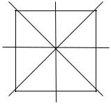
On a given plane P fix a point O and a line whose direction we shall call the horizontal. Now imagine a rigid square placed on P in such a way that its centre is at O and one side is horizontal. A symmetry of the square is defined to be a motion which leaves it looking as it did at the beginning, i.e. with its centre at O and one side horizontal. Clearly the following motions of the square are symmetries:

R: a 90° clockwise rotation about O

R′: a 180° clockwise rotation about O

R′′: a 270° clockwise rotation about O

H: a 180° rotation about the horizontal axis EF

V: a 180° rotation about the vertical axis GH

D: a 180° rotation about the diagonal 1–3

D′: a 180° rotation about the diagonal 2–4

We may compose (or multiply) two symmetries by performing them in succession. Thus, for example, the composite (or product) V.R of V and R is obtained by first rotating the square through 180° about GH and then through 90° about O. By experimenting with a wooden square, one can verify that this has the same total effect as D, rotation about the diagonal 1–3. Another way of checking this is by observing that both V.R and D have the same effect on each vertex of the square: V.R sends 2 into 1 by V and then 1 into 4 by R —hence 2 into 4, just as does D. Similarly, R.V is the result of a clockwise rotation through 90°, followed by a 180° rotation about a vertical

axis. It is easily checked that this is the same as D′, rotation about the diagonal 2–4.

Thus V.R ≠ R.V, so that composition is not commutative. It is, however, easy to see that it is associative, i.e., for any symmetries X, Y, Z we have

(X.Y).Z = X.(Y.Z).

If we compose the two symmetries R and R′′ in either order we see that the result is

a motion of the square leaving every vertex fixed: this is called the identity motion I, which we also regard as a symmetry. Given any symmetry X, it is clear that the motion X –1 obtained by reversing X is also a symmetry, and that it satisfies

X.X –1 = X–1.X = I.

We call X –1 the inverse of X.

We shall regard two symmetries as being identical if they have the same effect on (the vertices of) the square. Thus, in particular, since the inverse R–1 of R has the same

effect as R′′, we regard them as identical symmetries, and accordingly we may say that R′′ is the inverse of R.

We now have a list

{R , R′, R′′, H ,V, D, D′, I}

of eight symmetries of the square. This list in fact contains all possible symmetries, since any symmetry must carry the vertex 1 into any one of the four possible vertices, and for each such choice there are two possible symmetries, making a total of eight.

The set S of symmetries of the square accordingly has the following properties:

(1)the composite X.Y of any pair of members X,Y of S is a member of S, and for any X, Y, Z in S we have (X.Y).Z = X.(Y.Z);

(2)S contains an identity element I for which I.X = X.I = X for all X in S;

(3)for any X in S there is a member X –1 of S for which X.X–1 = X–1.X = I.

These three conditions characterize the algebraic structure known as a group. In general, a group is defined to be any set S—called the underlying set of the group—on which is defined a binary operation (usually, but not always, denoted by “.”) called

Hn = {0, 1,..., n –1}

can be turned into an additive group by means of the following prescription. For any p, q in Hn we agree that the “sum” of p and q, which we shall write p q, is to be the remainder of the usual sum p + q modulo n. It is then easy to check that Hn, with this operation , is an Abelian group, the group of remainders modulo n. In the case n = 5, for example, the “addition table” for is as follows:

0 1 2 3 4

00 1 2 3 4

11 2 3 4 0

22 3 4 0 1

33 4 0 1 2

44 0 1 2 3

In the case n = 2 we get the addition table for binary arithmetic:

0 1

00 1

11 0

Since, in H2, 0 represents the even numbers and 1 the odd numbers, this table is just another way of presenting the familiar rules:

even + even = odd + odd = even even + odd = odd.

There is a close connection between the additive group of integers and the remainder groups. In order to describe it we need to introduce the idea—one of the most fundamental in mathematics—of a function. A function, also called a transformation, map, or correspondence, between two classes of elements X and Y is any process, or rule, which assigns to each element of X a uniquely determined corresponding element of Y. The class X is called the domain, and the class Y the codomain, of the function. Using italic letters such as f, g to denote functions, we indicate the fact that a given function has domain X and codomain Y by writing

f : X → Y,

and say that the function f is from X to Y, or defined on X with values in Y. In this situation, we write f(x) for the element y of Y corresponding under f to a given element x of X: f(x) is called the image of x under f, or the value of f at x and x is said to be sent to f(x) by f. An old-fashioned notation for functions is to introduce a function f by writing y = f(x): here x is called the argument of f. We shall use this notation occasionally, and especially in Chapter 9.

It is sometimes convenient to specify a function f: X → Y by indicating its action on elements of its domain X: this is done by writing

x f(x).

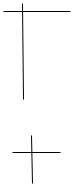
It is often helpful to depict a function f: X → Y by means of a diagram of the sort below, in which arrows are drawn from points in the figure representing the domain of the correspondence to their images in the figure representing its codomain.

y

y

Y

As examples of functions we have

xx + 1

xx

xx2

between, respectively, ] and itself, the set of rationals and the set of reals, and the set

of reals and the set of non-negative reals. A function is called one-one if distinct elements in its domain have distinct images in its codomain, and onto if every element of its codomain is the image of at least one element of its domain. A function which is both one-one and onto is called biunique, or a bijection, or sometimes a biunique correspondence. Thus a bijection is a function with the property that each element of its codomain is the image of a unique element of its domain. We see that the first function above is biunique, the second, one-one, and the third, onto.

Functions may also have more than one argument. Thus, for example, we may think of the process which assigns to each triple (x, y, z) of integers the number x5 + y5 + z5 as a function f from the set of triples of integers to the set of integers whose value at (x, y, z) is f(x, y, z) = x5 + y5 + z5.

Now fix an integer n ≥ 2. For each integer p in ] write (p) for its remainder modulo n: this yields a function

p (p)

between ] and Hn. This function is obviously onto, but not one-one since it is readily

seen that (p) = (q) exactly when p – q is divisible by n. It is now easy to check that we have, for any integers p, q,

For example, taking n = 5, p = 14, q = 13,

(14 + 13) = (27) = 2 = 4 3 = (14) (13).

Equation (1) tells us that the correspondence p (p) between and Hn transforms the operation + of ] into the operation of Hn, that is, it preserves the structure of the two groups. This fact is briefly expressed by saying that the function p (p) is a morphism (Greek: morphe, “form”) between ] and Hn.

The concept of morphism may be extended to arbitrary groups. Suppose given two groups G and H: let “ ” and “◊” denote the composition operations in G and H

respectively. Then a function f: G → H is called a morphism between G and H if, for any pair of elements x and y of G, we have

f(x y) = f(x) ◊ f(y).

The most familiar example of a morphism between groups arises as follows. Let Rp be the multiplicative group of positive real nunbers and let Ra be the additive group of all real numbers. The common logarithm4 log10x of a positive real number x is defined to be the unique real number y for which

10y = x.

The resulting function x log10x is then a morphism between Rp and Ra in view of the familiar fact that

log10(xy) = log10x + log10y.

This function has the further property of being biunique. A biunique morphism is called an isomorphism (Greek iso, “same”) and the groups constituting its domain and codomain are then said to be isomorphic. Thus log10 is an isomorphism between Rp and Ra; these groups are, accordingly, isomorphic. Isomorphic groups may be regarded as differing only in the notation employed for their elements; apart from that, they may be considered to be identical.

4Logarithms were introduced by John Napier (1550–1617) and developed by Henry Briggs (1561–1631). William Oughtred (1574–1660) used them in his invention of the slide rule, which was to become, by the nineteenth century, the standard calculating instrument cherished by engineers. Only recently has this elegant device—one of the most practical embodiments of the continuous—been superseded by that model of discreteness, the electronic calculator.

Rings and Fields

Another important type of algebraic system is obtained by abstracting at the same time both the additive and the multiplicative structures of the set Z of integers. The result, known as a ring, plays a major role in modern algebra. Thus we define a ring (a notion already introduced informally in Chapter 3) to be a system A of elements which, like Z, is an Abelian group under an operation of addition, and on which is defined an operation of multiplication which is associative and distributes over addition. That is, for all elements x, y, z of the ring A,

x.(y.z) = (x.y).z x.(y + z) = x.y + x.z (y + z).x = y.x + z.x.

If in addition we have always

x.y = y.x,

then A is called a commutative ring.

Naturally, Z with its usual operations of addition and multiplication is then a commutative ring: as such, it is denoted by ]. So, indeed, is the set {0, ±2, ±4,...} of even integers, as is the set of all multiples of any fixed integer n: this ring is denoted by ]n. Each of the remainder groups Hn for n ≥ 2 becomes a commutative ring—called a remainder ring—if we define the multiplication operation ◊ by

p ◊ q = remainder of pq modulo n.

The sets Q, R, and C of rational numbers, real numbers, and complex numbers, respectively, are obviously commutative rings. Earlier in this chapter we also encountered various example of rings of algebraic numbers, such as, for each integer n,

the ring ][√–n] consisting of all numbers of the form a + b√n, where a, b are integers. As an example of a noncommutative ring—that is, one in which multiplication is noncommutative—we have the set of n × n matrices with real entries for fixed n ≥ 1:

here the operations are matrix addition and multiplication.

Each of the rings Q, R, and C actually has the stronger property that its set of nonzero elements constitutes a multiplicative group. A commutative ring satisfying this condition is called a field (the concept of field has already been introduced informally in Chapter 3). Thus the rings of rational numbers, real numbers, and complex numbers

are all fields: as such, they are denoted by _, \, and ^. It is also easy to show that a

remainder ring Hn is a field exactly when n is prime.

Morphisms between rings are similar to morphisms between groups. Thus, given two rings A and B, we define a morphism between A and B to be a function f: A → B which preserves both addition and multiplication operations in the sense that, for any elements x, y of A, we have

Here the symbols +, . on the left side of these equations are to be understood as denoting the addition and multiplication operations in A, while those on the right side the corresponding operations in B. A biunique morphism between rings is called an isomorphism.

morphism between the rings Z and Hn. As another example, if m and n are integers ≥ 2 and n is a divisor of m, then the function from Hm to Hn which assigns to each integer < m its remainder modulo n is a morphism of rings. And the function x + iy x – iy is an

isomorphism of the field of complex numbers with itself (called conjugation).

Earlier in this chapter we encountered the notion of an ideal in rings of algebraic numbers. In general, given a commutative ring A, an ideal in A is a subset I of A such that, for any x, y in I and a in A, x+ y and ax are in I. Thus, for example, for any n, the

set Zn of integers divisible by n is an ideal in the ring of integers ]. There is a close

connection between ideals and morphisms of rings. Given a morphism of rings f: A → B, it is easily verified that the subset of A consisting of those elements a for which f(a) = 0—the kernel of f—is an ideal in B. For example, the kernel of the above

morphism p (p) from ] to Hn is ]n.

Ordered Sets

We are all familiar with the idea of an ordering relation, the most familiar example of which is the ordering of the natural numbers: 1 ≤ 2 ≤ 3 ≤ … . This relation has three characteristic properties:

It also has the property of

totality p ≤ q or q ≤ p for any p, q.

Now there are many examples of binary relations possessing the first three, but not the fourth, of the properties above. Consider, for instance, the relation of divisibility on the natural numbers. Clearly this relation is reflexive, transitive, and antisymmetric, but does not possess the property of totality since, for example, neither of the numbers 2 or 3 is a divisor of the other. Another example may be obtained by considering the “southwest” ordering of points on the Cartesian plane (see Chapter 7). Here we say that

one point with coordinates (x, y) is southwest of a second point with coordinates (u, v) if x ≤ u and y ≤ v, as indicated in the diagram

(u, v)

y (x, y)

A further example of such a relation is the inclusion relation on subsets of a given set. Here we suppose given an arbitrary set U of elements: any set consisting of some (or all) elements of U is called a subset of U. We count the empty set, denoted by , possessing no elements at all, as a subset of any set. The collection of all subsets of U is called the power set of U and is denoted by Pow(U). Thus, for example, if U consists of the three elements 1, 2, 3, Pow(U) contains the eight different sets {1, 2, 3}, {1, 2}, {1, 3}, {2, 3}, {1}, {2}, {3}, . Given two subsets X and Y of U, we say that X is included in Y , written X Y, if every element of X is also an element of Y, as indicated by the diagram

Y

X

It is now readily verified that the relation of inclusion between subsets of an arbitrary set U is reflexive, transitive, and antisymmetric, but does not possess the totality property if U has more than a single element. Note that inclusion is antisymmetric because two sets with the same elements are necessarily identical.

These examples lead to the following definition. A partially ordered set is any set P equipped with a binary relation ≤ which is reflexive, transitive, and antisymmetric: in

this event the relation ≤ is called a partial ordering of P. If in addition the relation ≤

satisfies the totality principle then P is said to be totally ordered. As examples of partially ordered sets we have all those mentioned in the previous paragraph, viz., the natural numbers with the divisibility relation, the points on a plane with the south-west ordering, and the power set of a set with the inclusion relation. Other important examples of partially ordered sets are the collections of all subgroups of a given group, or ideals of a given commutative ring, together with the inclusion relation. As examples of totally ordered sets we have the familiar sets of natural numbers, rational numbers, and real numbers with their usual orderings.

For any partial ordering ≤, we write q ≥ p for p ≤ q and define p < q to mean that p ≤ q but p ≠ q, and we say that q covers p if p < q but p < r < q for no r.

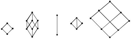
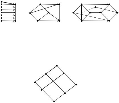
Partially ordered sets with a finite number of elements can be conveniently represented by diagrams. Each element of the set is represented by a dot so placed that the dot for q is above that for p whenever p < q. An ascending line is then drawn from

p to q just when q covers p. The relation p ≤ q can then be recovered from the diagram

by observing that p < q exactly when it is possible to climb from p to q along ascending line segments of the diagram. Here are some examples:

y

The first of these represents the system of all subsets of a two element set; the second, that of all subsets of a three element set; the third, the numbers 1, 2, 4 under the divisibility relation; the fourth, the numbers 1, 2, 3, 5, 30 under the divisibility relation; the fifth, the nine points (0, 0), (1, 0), (2, 0), (0, 1), (1, 1), (2, 1), (0, 2), (1, 2), (2, 2) in the plane with the southwest ordering.

Just as for groups and rings, we can define the concept of morphism between partially ordered sets. Thus a morphism between two partially ordered sets P and Q is a function f: P → Q such that, for any p and q in P,

p ≤ q implies f(p) ≤ f(q).

(Here the left-hand occurrence of the symbol “≤” ignifies the partial ordering of P, and

the right-hand occurrence that of Q.) A morphism between partially ordered sets is an order-preserving function.

Here are some examples of morphisms between partially ordered sets:

1)the function x x2 from the totally ordered set of natural numbers to itself;

2)the function x ½x from the totally ordered set of rationals to itself;

the southwest ordering to the totally ordered set of real numbers;

4) the function x|→ [x] from the totally ordered sets of reals to that of integers, where, for each real number x, [x] denotes the greatest integer not exceeding x;

5) the function X X* from the power set of the real numbers to that of the

integers, where, for each set X of real numbers, X* denotes the set of integers contained in X;

6) the following functions between finite partially ordered sets indicated by the diagrams

Lattices and Boolean Algebras

Certain of the partially ordered sets we have considered, for example that given by the diagram:

t

r

p yq

s

b

have a special, and important, property. To describe it, consider two typical elements p and q. We see then from the diagram that the element marked r is the least element ≤

both p and q in the sense that any element x with this property must satisfy r ≤ x. Similarly, the element s is the greatest element ≤ both p and q in the sense that any element y with this property must satisfy y ≤ s. The elements r and s are called the join

and meet, respectively, of p and q. It is easy to see that any pair of elements of this particular partially ordered set has a join and a meet in this sense.

This example suggests the following definition. A lattice is a partially ordered set P in which, corresponding to each pair of elements p, q there is a unique element, which we denote by p q and call the join of p and q, such that, for any element x,

p q ≤ x exactly when p ≤ x and q ≤ x;

and also a unique element, which we denote by p q and call the meet of p and q, such that, for any element x,

x ≤ p q exactly when x ≤ p and x ≤ q.

Lattices constitute one of the most important types of partially ordered set. Any totally ordered set is obviously a lattice, in which join and meet are given by:

p q = greater of p, q, p q = smaller of p, q.

The set of positive integers with the divisibility relation is also a lattice in which join and meet are given by

p q = least common multiple of p, q,

p q = greatest common divisor of p, q.

The set of points in the plane with the southwest ordering is a lattice, with join and meet given by:

(x, y) (u ,v) = (max(x, u), max(y, v)),

(x, y) (u ,v) = (min(x, u), min(y, v)).

For any set U, its power set Pow(U) is also a lattice with join and meet given by

It is customary to write X Y, X ∩ Y for the union and intersection of X and Y.

The lattice Pow(U) has several important additional properties that we now describe. First, it satisfies the distributive laws, that is, for any X, Y, Z in Pow(U) we have

X ∩ (Y Z) = (X ∩ Y) (X ∩ Z),

X (Y ∩ Z) = (X Y) ∩ (X Z).

These equalities are readily established by the use of elementary logical arguments showing that the sets on either side have the same elements. Secondly, it has least and largest elements: the empty set is least in that it is included in every subset of U, and

the set U itself is largest since it includes every subset of U. Finally, Pow(U) is complemented in the sense that, for any subset X of U, there is a unique subset X′of U called its (set-theoretic) complement such that

X X′= U, X ∩ X′= .

Here X′—which is sometimes written U – X—is the subset of U consisting of all

elements of U which are not in X.

A lattice satisfying these additional conditions is called a Boolean algebra. Thus a Boolean algebra is a lattice L which is

(1) distributive, that is, for any p, q, r in L,

p (q r) = (p q) (p r),

p(q r) = (p q) (p r);

(2)complemented, that is, possesses elements t (“top”) and b (“bottom”) such that b ≤ p ≤ t for all p in P, and corresponding to each p in P there is a (unique) element p′ of P for which

p p′= b, p p′= t.

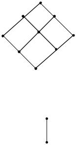
Thus every lattice Pow(U) is a Boolean algebra. On the other hand, for example, the nine element lattice

while distributive, is not a Boolean algebra because, as is easily seen, its central element has no complement.

The two element lattice

true

false

is obviously a Boolean algebra since it represents the lattice of all subsets of a one element set. It plays a particularly important role in logic as it also represents the system of truth values. In classical logic propositions are assumed to be capable of assuming just two truth values true and false. These are conventionally ordered by placing false below true (so that false is “less true” than true): the result is the two element Boolean algebra above, which is accordingly known as the truth-value algebra.

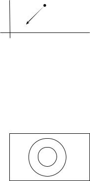
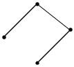
The four element lattice of all subsets of a two element set is a Boolean algebra which, interestingly, also represents the system of human blood groups. Given

any species S, define, for individuals s and t of S, s ≤ t to mean that t can accept— without ill effects—transfusion of s's blood. Then the relation ≤ is clearly reflexive and (presumably) transitive, but not antisymmetric. We call individuals s and t of S equivalent if both s ≤ t and t ≤ s: thus equivalent individuals are mutual blood donors.

Equivalent individuals are said to be members of the same blood group. Accordingly a blood group is the class of individuals equivalent to a given one. In 1901 the Austrian scientist Karl Landsteiner (1868–1943) discovered that the human species comprises four such blood groups: these are customarily denoted by O, A, B, and AB. They form a

partially ordered set in a natural way: for any blood groups X and Y we define X ≤ Y to mean that s ≤ t for any individuals s in X, t in Y. The resulting partially ordered set is the four element Boolean algebra

AB

A B

O

with bottom element O—the group of universal donors—and top element AB —the group of universal recipients. It would seem then appropriate to call the four element Boolean algebra the blood group algebra or the Landsteiner algebra.

The concept of morphism can be defined for lattices and Boolean algebras in the natural way. Thus, a function f is a morphism between two lattices L and L′ if for any x, y in L we have

f(x y) = f(x) f(y), f(x y) = f(x) f(y).

If L and L′are Boolean algebras, f is a Boolean morphism if in addition it satisfies, for any element x of L,

f(x*) = f(x)*,

where x* denotes the complement of x.

It is easy to check that the first two correspondences given in 6), p.105, are lattice morphisms but the third is not (also that the partially ordered sets concerned are

The most important fundamental results in the theory of (distributive) lattices and Boolean algebras involve the concept of isomorphism, where two lattices or Boolean algebras are said to be isomorphic if there is a biunique morphism between them. Let us define a lattice of sets to be a lattice whose members are sets and in which meet and join are set-theoretic intersection and union, respectively, and a Boolean algebra of sets to be a Boolean algebra whose members are sets and in which meet, join and complement are set-theoretic intersection, union, and complementation, respectively. Then we have the following representation theorem (due to M. H. Stone): any distributive lattice, or Boolean algebra, is isomorphic to a lattice, or Boolean algebra, of sets. This result shows that the axioms for distributive lattices or Boolean algebras are an “abstract” characterization of the laws governing the set-theoretic operations, first identified by Boole, of union, intersection, and complementation.

Category Theory

Each of the types of structure—groups, rings, fields, partially ordered sets, lattices, Boolean algebras—we have introduced has an associated notion of morphism, or “structure-preserving” function. In studying these and other mathematical structures, mathematicians came to realize that the idea of morphism between structures was no less important than the idea of structure itself. It was essentially for this reason that S. Eilenberg (1914–1998) and S. Mac Lane created, in 1945, category theory, a general framework for mathematics in which the concepts of mathematical structure and morphism are accorded equal status.

In order to motivate the definition of category let us return to groups and morphisms between them. The first and most important fact we note about these morphisms is that they can be composed. Thus, suppose we are given two morphisms f: G → H and g: H→ J, such that the codomain H of f coincides with the domain H of G. Then we can define a composite morphism g f : G → J by

(g f )(x) = g(f(x))

for x in G. It is easy to see that composition in this sense is associative, that is, for morphisms f: G → H, g: H → J, h: J → K we have

h (g f ) = (h g ) f .

110 CHAPTER 6

Another fact is that the identity function x x on each group G is a morphism between

G and itself: it is called the identity morphism on G and written idG. Clearly identity morphisms have the following property: for any morphism f: G → H,

f idG = idH f = f .

These features provide the basis for the definition of a category. Thus a category consists of two collections of entities called objects and arrows: here objects are to be thought of as the formal counterparts of mathematical structures and arrows as the formal counterparts of morphisms between them. Each arrow f is assigned an object A called its domain and an object B called its codomain: this fact is indicated by writing f: A → B. Each object is assigned a morphism idA: A → A called the identity arrow on A. For any pair of arrows f: A → B, g: B → C (i.e., such that the domain of g coincides with the codomain of f), there is defined a composite morphism g f: A → C. These prescriptions are subject to the laws of associativity and identity, viz., given three

Thus we obtain the category of groups whose objects are all groups and whose arrows are all morphisms between them. Similarly, we obtain the categories of rings, partially ordered sets, lattices, and Boolean algebras: the objects of each of these categories are structures of the sort specified and the arrows morphisms between such structures. Another important category is the category of sets, with arbitrary sets as objects and arbitrary functions as arrows.

The fact that any type of mathematical structure determines a corresponding category has led mathematicians to regard category theory as the natural framework for describing the general characteristics of mathematical discourse. By providing a means of expressing the features common to the many branches of mathematics that have appeared in the twentieth century, category theory has come to play an important role in preserving its unity.